

Key Points
It makes sense, intuitively, that equity factor performance and stages of the economic cycle are linked. We analyze the relationship across six geographic regions and over all four economic stages of growth, slowdown, recession, and recovery to discover the historical nature of that relationship.
The majority of the eight factors (including the market factor) that we examine produce a positive and significant total return over the full study period. Three components drive the total return: changes in fundamentals, changes in valuation, and valuation rebalancing.
Fewer factors produce meaningful returns when we consider a factor’s structural return, the portion of the return that is indefinitely repeatable. Over the study period, the value factor has the highest structural return.
The higher economically leveraged factors—market, size, value, and illiquidity—perform better during the positive economic stages of recovery and growth, and perform poorly during the negative economic stages of recessions and slowdowns. The opposite applies to the less economically leveraged factors—low beta and profitability.
We find that the relationship between factors and economic stages generally fits with intuition. Because data are limited, however, we do not have sufficient observations of economic significance, leaving us unable to call it a “committed” relationship.
The economy has very real implications in our daily lives. Our jobs, spending, and personal well-being are all tied to its ups and downs. When economic times are good, we feel good. When economic times are bad, it gets us down. The same is true of the capital markets. When economic times are good, it feels like the market has no bound on the upside. During tough economic times, during recessions, it seems everything piles up against the market, and returns suffer. Simply, the state of the economy matters. It has consequences not only in our everyday decisions, but also in how the capital markets behave.
Factor investing has become a valid choice for investors looking to implement the shares slice of their portfolio. No doubt, the super-secular theme of declining management fees has made these systematic, rules-based strategies an attractive alternative to traditional active management. As investors implement factor strategies more often, it becomes more important for them to understand factors’ cyclical tendencies. Here, we look at the performance of different factor portfolios across six regions and four economic stages to determine if, and how much, the economy has impacted past factor performance.
Market Factor Across the Economic Cycle
Superannuation funds have an overwhelmingly large allocation to shares given the theoretical and empirical observations of long-horizon equity excess returns over fixed interest. The market portfolio, the return on a broad-based and capitalization-weighted portfolio in excess of the risk-free cash rate, through June 2020 has returned 5.6% a year in the United States (since July 1969) and 7.7% a year in Australia (since July 1989), using data from CRSP/Compustat and Worldscope/Datastream.
Sharpe (1964) is often credited as being the first to publish research on the market as an equity factor. Although investors have constructed broad, market-based portfolios for some time, it was not until the last month of 1998 that the US market portfolio (since July 1969) produced a statistically significant positive return. The significance of the market factor did not last long, however, and would have to wait until March 2013—a few months short of a full 45 years—to again record a significant positive return. The Australia market, with higher return and risk than the US market, spent the last few decades oscillating between a significant and an insignificant positive return.
We point out the instability of the market return, the first documented factor return, to show that to gain statistical confidence of a positive return, we need decades, preferably out of sample. For most markets, we do not have that luxury. Hence, the power of these tests, the ability to discover a true positive factor return, is weak.
We can gain stronger results for the market portfolio by combining geographic observations. We dispense with the traditional approach of only using factor returns from a given country, and extend our database to six regions composed of four countries—United States, United Kingdom, Japan, and Australia—and two groups of countries—Europe and the emerging markets, and calculate a market factor return for each of the six, over a total of 2,352 monthly data points.
We observe an average annualized market factor return of 5.8% a year. Exposure to this factor, the primary and most dominant source of risk for all but the most conservative portfolios, has become the default risk of long-horizon portfolios. Consequently, investors have developed a very long-term horizon to wait out the performance of the market factor. Further, because investors tend to have an equity bias, this periodic underperformance does not greatly impact relative performance comparisons, and thus the career risk of being, as John Maynard Keynes quipped, the most dangerous place in investing, namely, being “wrong and alone.”
Across the four economic stages, two major themes are at play: economic leverage and momentum.Historically, the market factor has significantly underperformed in a seemingly repetitive fashion. In other words, the market factor earns different returns over the stages of the business cycle. Research Affiliates’ analysis shows this to be true. Our analytical framework defines four economic stages using information on real gross domestic product (GDP) and the OECD system of Composite Leading Indicators (CLIs):1
Recession: two consecutive quarters of negative growth
Slowdown: nonrecessionary below-trend growth
Recovery: post-recessionary (24 months) above-trend growth
Growth: remaining months (after the first 24) of above-trend growth
The growth stage is the most common of the four stages across the six regions, encompassing 40% of the total 2,500 months in the study period. Slowdowns follow closely at 36% of months. Because both growth and slowdown periods are defined relative to trend real-GDP growth, the nearly even split is not surprising. The split also highlights that slowdown periods tend to be slightly larger in magnitude than growth periods. The more economically impactful periods of recessions and recoveries make up the remaining 10% and 15% of months, respectively.
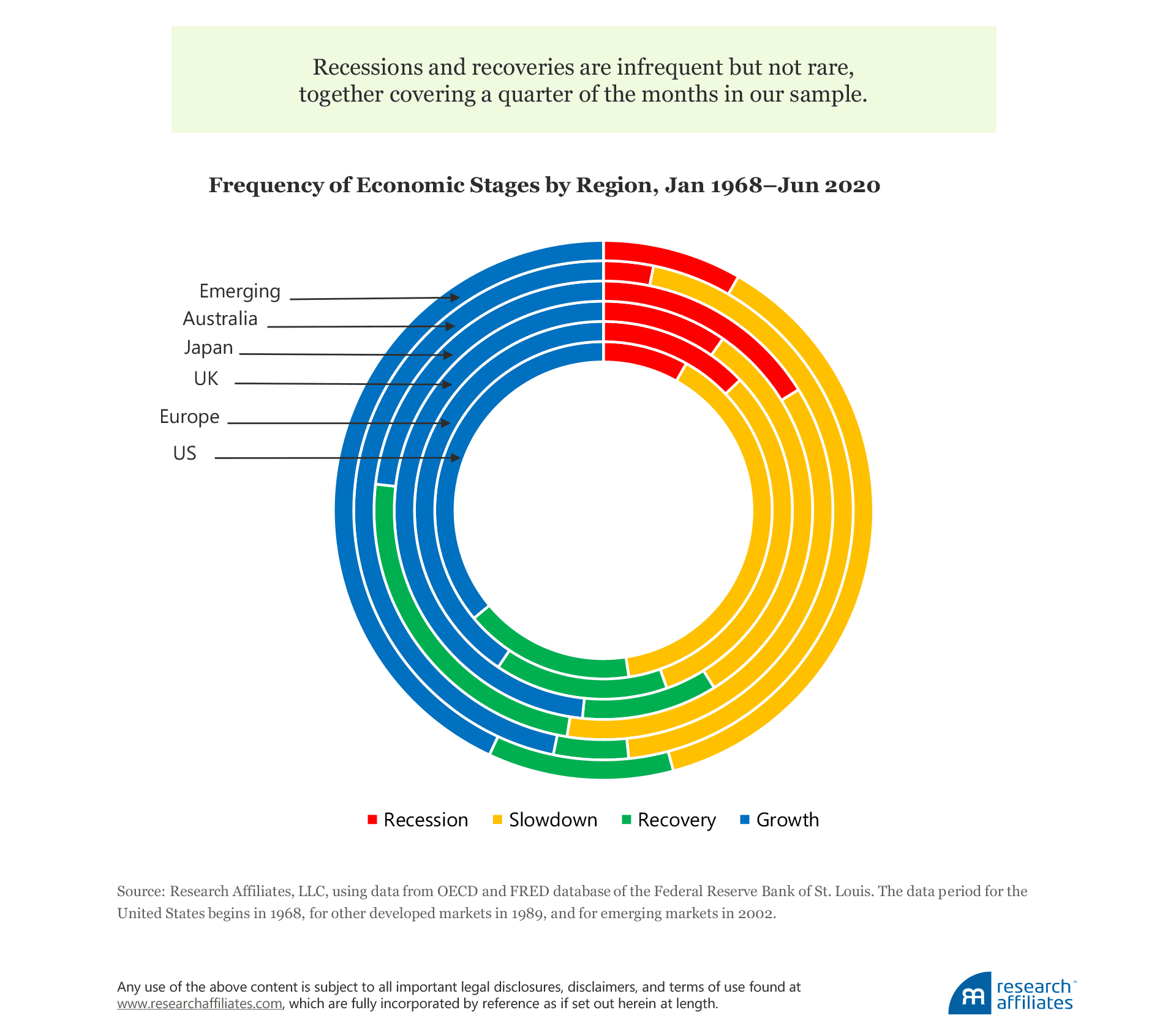
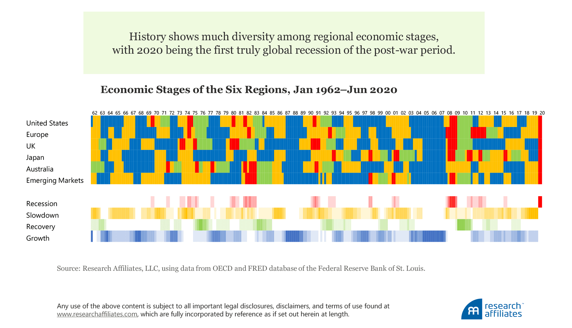
Over each region’s period of analysis, its respective economic stages are distributed differently to the economic stages of the other regions. While we can reliably construct historical data for each of the economies, we are limited by the consistently constructed factor return data. Therefore, the US data set begins in 1968, data for the other developed markets start in 1989, and emerging market data date to 2002. Keeping the variation among data sets in mind, of the six regions, Japan has the highest proportion of recessions and recoveries, composing 43% of the nation’s data set.
Japan did not experience a recession during its post-World War II economic recovery, but after an asset bubble of extraordinary proportions burst in 1992, the nation suffered a chain of recessions and recoveries. In stark contrast, Australia has the lowest proportion of recessions and recoveries, composing only 8% of the nation’s data set. Before 2020, Australia’s last recession was in the early 1990s. The nation avoided both the late 1990’s tech tumble and the 2008 credit crisis that plagued all other regions in our sample.
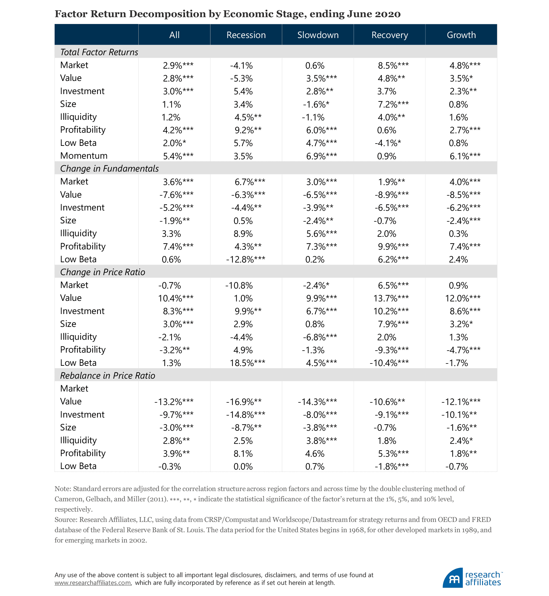
So how does the market factor, differing as it does across multiple regions and time periods, perform across different economic stages? We start by considering performance coincident with the economic stage, tacitly assuming that markets are not already looking ahead to the next stage of the cycle. Unsurprisingly, the market factor underperforms during recessions with an annual return of −4.1%. Over slowdowns, which may or may not migrate to a recession, the market return is 0.6%. Also, unsurprisingly, recovery and growth stages produce the best results with returns of 8.5% and 4.8% a year, respectively.
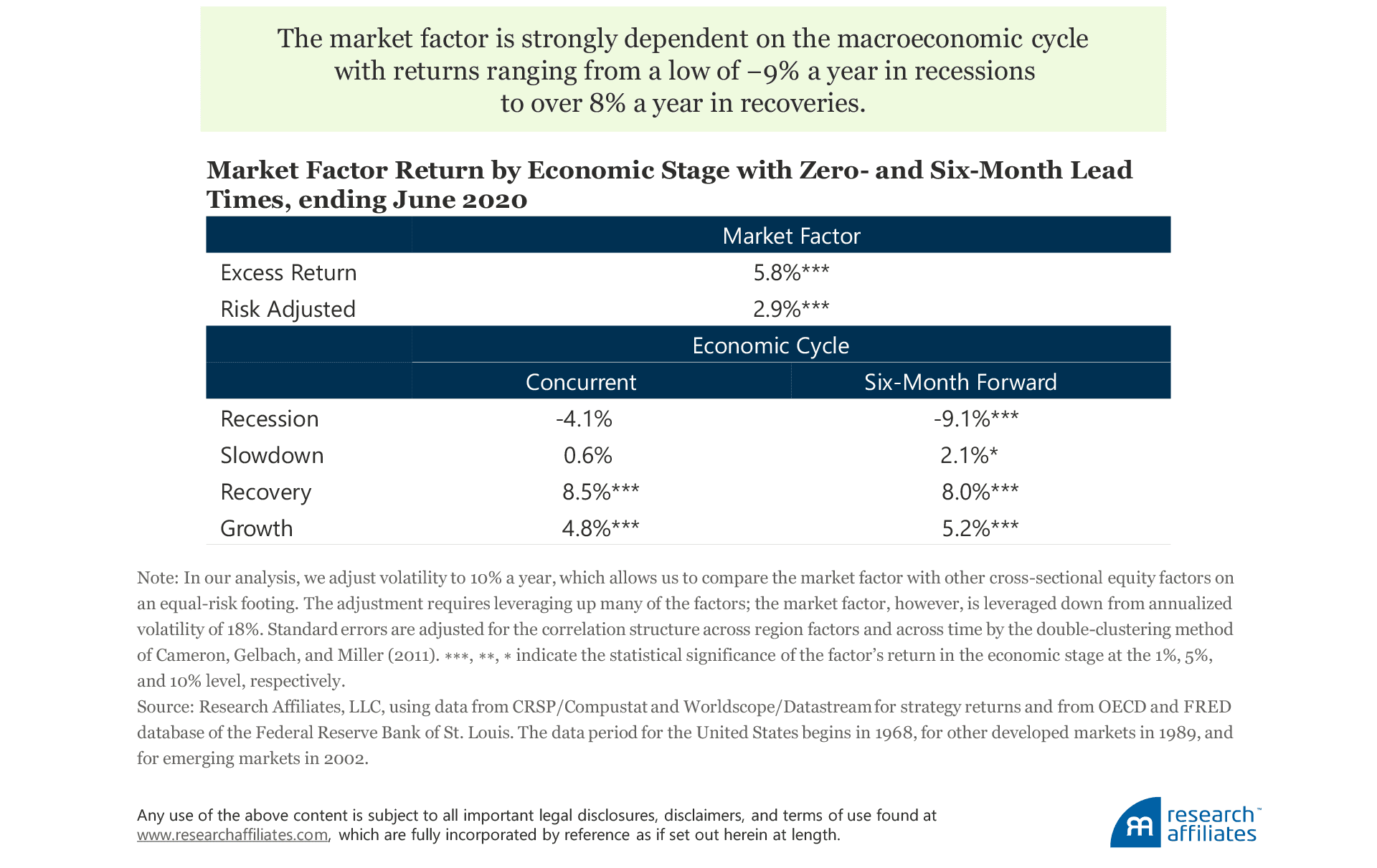
Of course, markets are discounting mechanisms as participants anticipate economic conditions. Although the concurrent economic stage requires some degree of forecasting, capital markets may already be declining ahead of an actual recession or advancing ahead of an actual recovery. Therefore, with a more realistic performance period that looks at the economic stage six months ahead, the excess return of the market factor falls to –9.1%, and the slowdown, recovery, and growth excess returns all increase to 2.1%, 8.0% and 5.2% a year, respectively. The market factor returns are significantly different from each other in all four stages for at least one of the concurrent or six-month economic lead models.
A Factor’s Actual and Structural Return
But does the economic stage matter in a substantive way to the return of other factors within the cross-section of the shares market? For the remainder of our discussion, we will focus on known factors that produce positive and significant non-zero annual returns. Of course, a “known” factor is in the eye of the beholder as evidenced by the hundreds of factors “identified” to date in the literature, many of which will likely prove to be spurious (Harvey and Yan, 2019).
Thus, we limit our analysis to factors that either meet, or come close to, the Hsu-Kalesnik-Viswanathan (HKV) (2015) framework for robustness. Namely, factors should be 1) grounded in a long and deep academic literature, 2) robust across definitions, and 3) robust across geographies. HKV also consider transaction costs, providing a more realistic view of how factors perform in live portfolios. Our analysis covers the market, value, investment, profitability, and momentum factors. In addition, we analyze several factors that may not display positive long-term returns, but have significant return differentiation between economic cycles; in this category we include the size, illiquidity, and low beta factors.
All of the HKV framework factors show a long-term return significantly different from zero.2 The long-term returns of the size, illiquidity, and low beta factors are not meaningfully significant. The low beta factor is not constructed as beta neutral, but if we regress the market factor out of the low-beta return series, the alpha, or residual, is significantly positive.
We find that annual factor returns tend to be significant if they are 2% or higher, but the exact number fluctuates based on the factor’s volatility. A test has power if it is able to identify a factor as significant when it has a truly positive return. To find a factor significant, the magnitude of its return needs to be sufficiently large given the size of the data set. If a factor’s true return is positive, but smaller than the relevant magnitude for the size of the data set, more independent data points are necessary to increase the power of the test.
Factor returns, including the market factor, are influenced over time by changing valuations.3 We can decompose equity factor returns by calculating 1) the return due to changing valuations and 2) the return due to changing fundamentals. For our analysis, we use a broad measure of fundamentals, the same metric used for the composite value factor: the average of book value, sales, earnings, and dividends. The price ratio, or valuation, is therefore the average ratio of a security’s price to its per share fundamentals. Arnott et al. (2020) provide more detail on the decomposition of a factor’s return into changes in fundamentals and changes in price ratio.
A value strategy earns a positive long-term return by investing in securities that have below-average expected growth. Hence, we would expect the value factor to have a negative change in fundamentals and, in fact, we see that over our sample period the value factor’s long portfolio grew 7.6% a year less than its short (or growth) portfolio. While this may not appear to bode well for the factor, over the same period the valuation ratios of the long securities rose 10.4% a year faster than the securities in the short portfolio. A quick calculation shows a 2.8% annualized return for the value factor over the study period.
In contrast, some factors have faster growth in fundamentals and decreasing valuations, such as the illiquidity and profitability factors. Both of these factors invest in higher-priced, rapidly growing companies in a bet that the faster growth in fundamentals will compensate investors for the extra price they pay for them.4
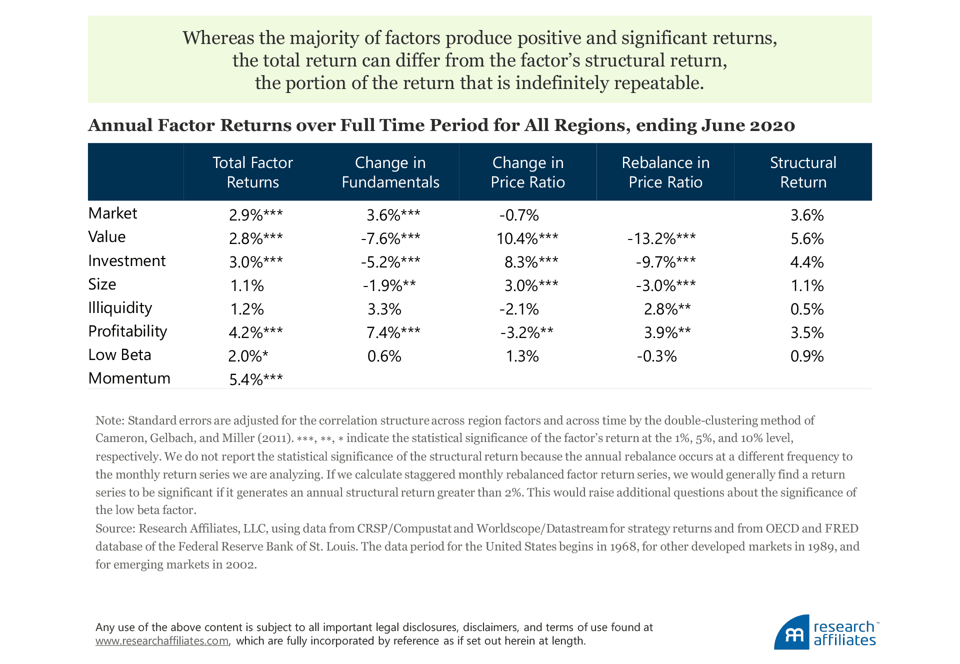
All factor portfolios, except for the market portfolio, need to be rebalanced regularly. The rebalancing process replenishes the portfolios with securities that meet the criteria of the factor. An important metric in analyzing a factor’s return is how much of the price ratio is replenished in the rebalancing. For example, in our study, in the value factor’s annual rebalancing, the average price-ratio replenishment was 13.2%. In contrast, when the profitability factor portfolios rebalanced, the average increase in price ratio was 3.9%. Marrying the fundamental growth of a factor with the rebalancing price ratio gives a better indication of the long-term structural return of a factor.
The structural component of a factor’s return will be higher if the reduction in the price ratio from rebalancing is higher than the observed change in the price ratio; this was the case for the market, value, and investment factors. Alternatively, over the study period, the size, illiquidity, profitability, and low beta factors experienced changes in the price ratio from rebalancing that were lower than the returns derived from changes in the price ratio. For these last four factors, the historical return benefited from a one-off valuation uplift, but the long-term repeatable structural return remained below that of the full-period factor return. In another publication, we will expand on the concept of factor valuation, especially as it relates to producing signals for tactical allocations amongst the factors.
The Power of a Regression
Kalesnik and Polychronopoulos (2020) examine factor returns in the United States during recessions and recoveries. We expand their work to include all four economic stages. You may ask—why has this analysis not been done (rigorously) before? It is, as is often the case, a data problem. Our analysis considers the dependency of factor returns on the different economic stages, similar to the analysis presented earlier for the market factor. To do this we must subdivide the factor return series.
Our historical experience, the time series of returns, is all we have to analyze. As explained earlier, in general we have the fewest data points for recessions, with even fewer recessionary periods in Australia. Recoveries are also relatively rare, because they follow recessions. Growth and slowdown periods are the most common, each composing about 40% of the data points. Recessions, not only being the rarest stage, also have the largest return volatility at 12.8% a year, with slowdowns having the second most volatile returns at 9.9% a year. Recovery and growth periods both produce an average volatility of 8.7% a year.
When we divide the data set into four subsets that correspond to the four economic stages of a business cycle, we lose observations and therefore explanatory power. This deficiency is particularly acute for the recessionary stage, which has the smallest number of observations and highest factor volatilities. For example, with our current data set we would generally need to have a difference in recessionary return greater than 5% a year versus the baseline return to discriminate the return from the background noise of random luck.
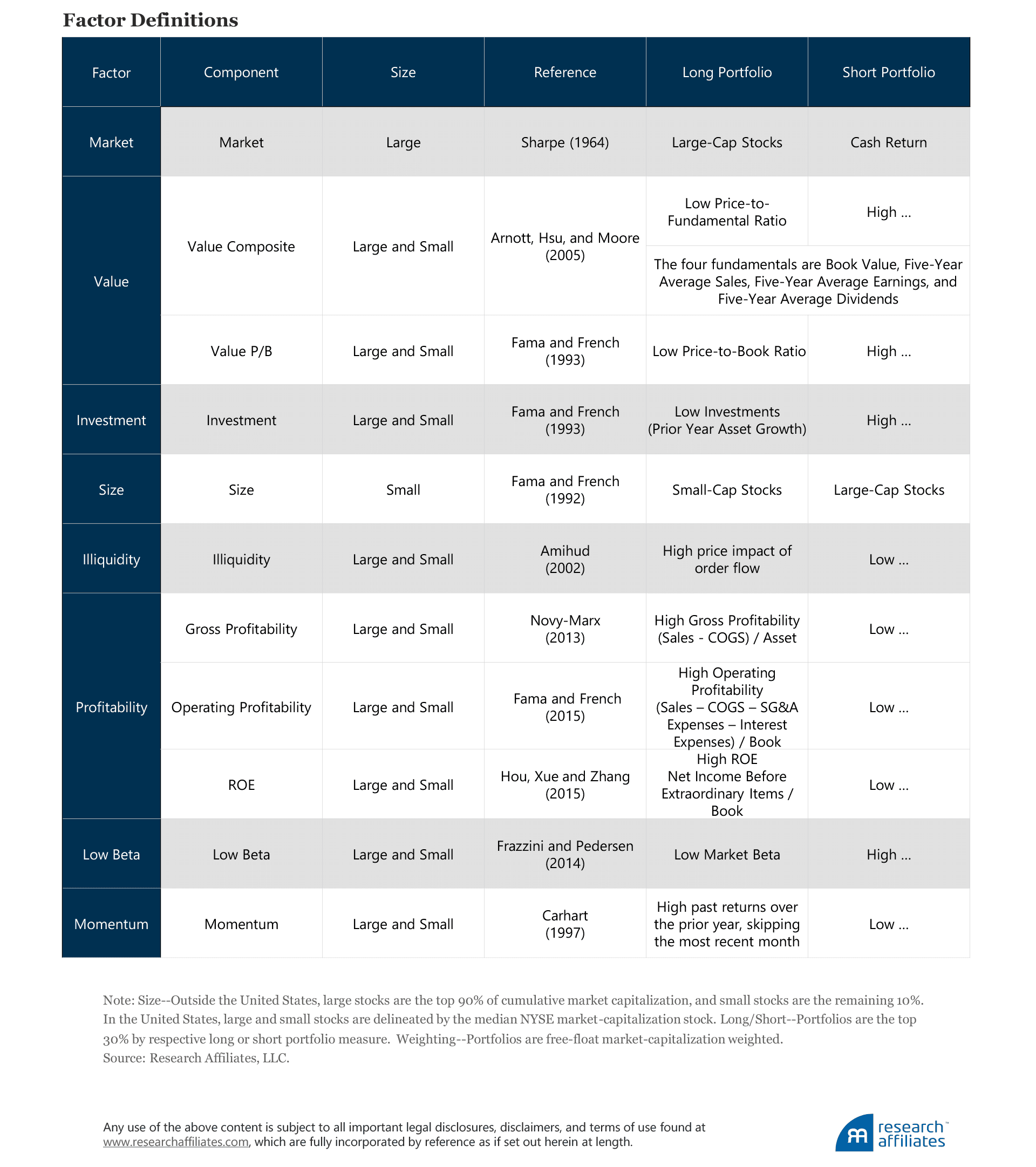
As explained earlier for the market factor, we extend our data set regionally in order to increase the data pool and the power of our regressions. In order to generate multi-regional factor portfolios, we need to calculate the factor portfolios in a consistent manner inter-regionally. The methodology we use to construct these factor portfolios is described in the appendix.
Factor Performance by Economic Stage
Most long-horizon investors have a persistent equity bias. Thus, the performance of the market factor across economic cycles is less problematic in relative comparisons, such as the regularly published superannuation tables. If allocations to the market factor are similar, a plan’s or fund’s equity allocation is unlikely to land it in the dreaded bottom decile. This observation is less applicable to factors within equities, however, which are more likely to be judged using the same three-to-five-year performance cycle relied on for decades in making hiring/firing decisions of active managers. Thus, long-horizon investors have an incentive to better understand and act on factor variations across shorter time horizons. The business cycle is often a first place to start. Our objective for the remainder of this article is to understand factor performance across the business cycle.
We calculate and present returns as the difference between the factor’s return in a given economic stage and all other returns not of that stage. We ask the question: “Does the market factor return differ in a recession to its return not in a recession?” The answer is “yes.” During a recession with a six-month lead, the market factor returns 13.1% less than in nonrecessionary months, significant at the 1% threshold. We repeat the analysis across all factors, all four economic stages, and for both the concurrent and six-month economic lead time. The results, although not uniformly significant, support our basic proposition that the economic stage impacts factor returns.
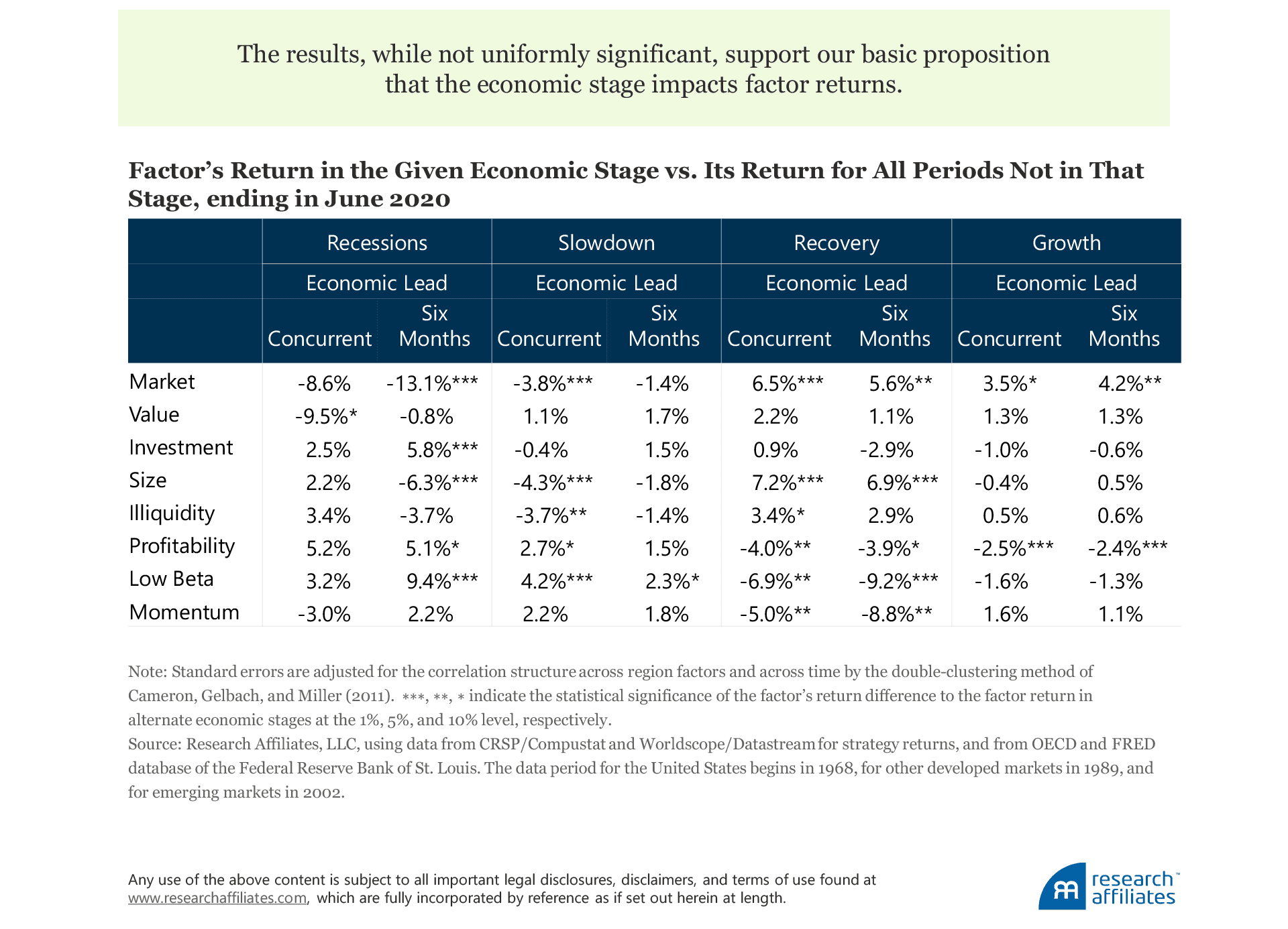
We make some observations of the recessionary periods that are consistent with our intuition and with economic theory. First, the market, value, and size factors underperform, and we see better-than-average returns for the low beta, profitability, and investment factors. Economic theory leads us to believe that companies leveraged to the economic cycle, such as value and small companies, will perform poorly when the economic environment is poor. The average company, and similarly the market factor, should also perform poorly, a combination of increasing discount rates and falling profits. In contrast, companies with lower leverage of the economic environment, as represented in the long portfolio of the low beta, profitability, and investment factors, do better.
We can think of a slowdown as a mini-recession, a period when growth is below trend, but does not slip into negative territory for two quarters in a row. Consistent with the concept of a mini-recession, we observe outperformance by the low beta factor and underperformance by the size, illiquidity, and market factors, but at a much-reduced magnitude—and here the mini-recession idea ends, with both value and momentum factors doing well. Momentum performs well because slowdown is not the reversal of economic fortunes, just a pause. Likewise, value companies are levered to the economic cycle, but priced cheaply enough to weather a slowdown. Unlike recessions, most of the explanatory power of a slowdown occurs when considering the concurrent (or zero-month lead) economic stage.
Recoveries are characterized by above-trend growth following a recession. Given the economic advantage of a recovery, factors that have higher economic leverage should do better. Therefore, factors that suffer during a recession unsurprisingly do well in recoveries. The market, value, size, and illiquidity factors all perform well. Not surprisingly, the economically conservative factors, such as low beta and profitability, perform poorly. Because recoveries follow recessions and are defined by a reversal of economic fortunes, the momentum factor performs poorly, experiencing a delay in recomposing itself to adjust to the new economic reality. The return significance is similar across both the concurrent and six-month-lead recoveries.
The growth stage, the most common, is a period of above-trend economic growth that does not follow a recession. Growth periods are characterized by prosperity, such as the disinflationary economic status quo most of the world has enjoyed over the last 40 years. Growth periods are generally good for shares and, therefore, for the market factor. Alternatively, the low beta and quality factors typically underperform.
Factor investing, like the Facebook relationship tag, is 'complicated' across the economic cycle.Across the four economic stages, two major themes are at play. First, economic leverage divides the higher economically leveraged factors of market, size, value, and illiquidity from the less economically leveraged factors of low beta and profitability. The pro-leveraged factors perform better during the positive economic stages of recovery and growth, and perform poorly during the negative economic stages of recessions and slowdowns. The opposite applies for the anti-leveraged factors of low beta and profitability.
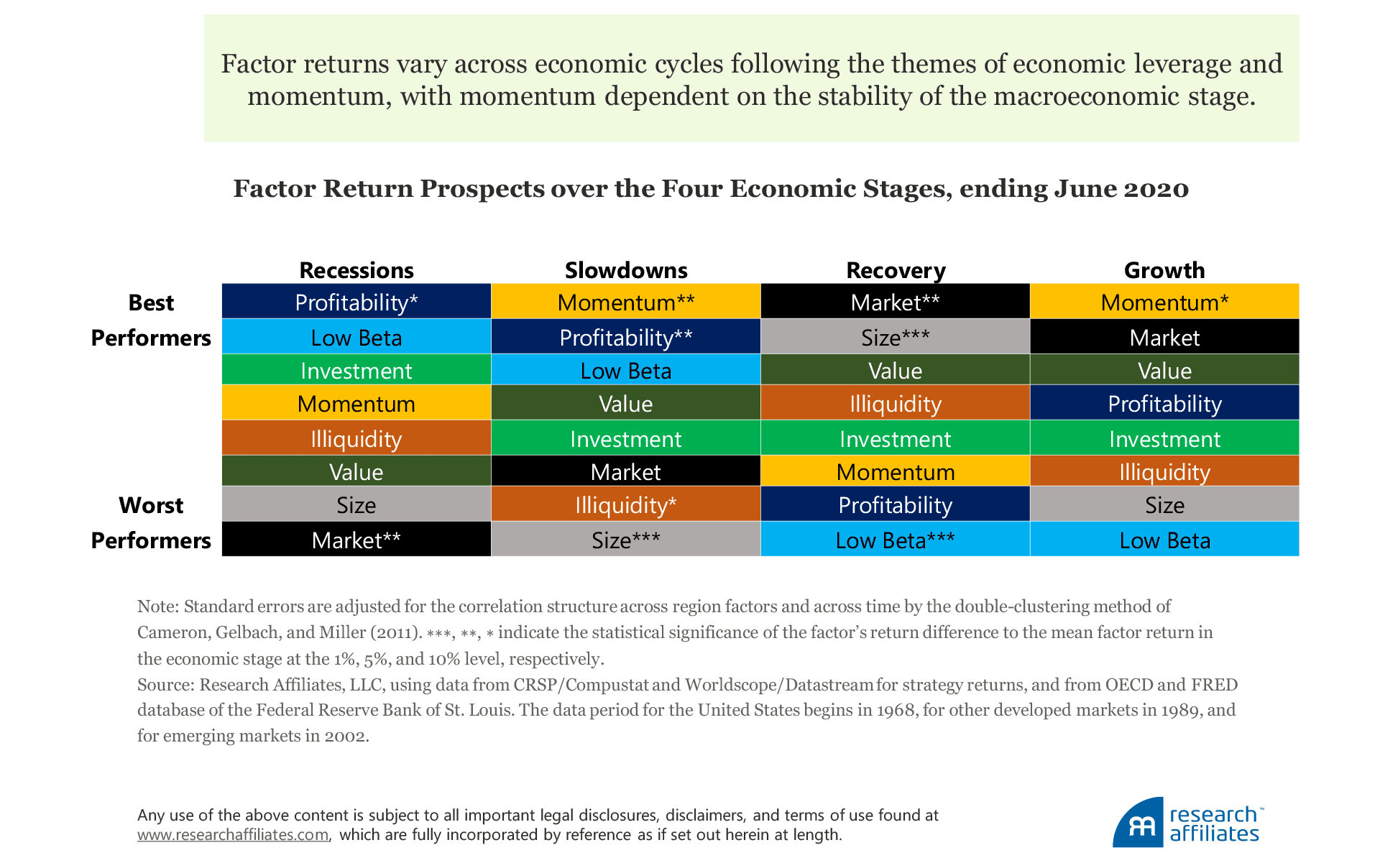
The second theme is momentum, which performs better during the longer-lasting stages of slowdown and growth. In the shorter and more economically significant, but less sustained, recession and recovery stages, momentum produces poor performance outcomes.
It’s a Complicated Relationship
From the early days of modern investment theory, Markowitz (1952) outlined the importance of the economy as a driver of investment gains and losses. Clearly, the return of the market factor depends on the state of the economy. In our study, the market factor’s performance mirrors, at a 95% statistically significant difference in returns, three of the four stages (considering a six-month lead)—with the growth period as the exception5—but three out of four ain’t bad! We therefore could say the market factor is “married” to the economic cycle.
Our results demonstrate that conclusions about the performance of various factors across the economic cycle seem, in most cases, to be consistent with the intuition of experienced investors. Whereas the factor results across the economic cycle differ in a way that is consistent with our intuition, we find fewer than expected observations of economic significance. Although the profitability and low beta factors have a record similar to the market factor, in three of the four stages performance significantly differs, and for the value factor, no stage is significantly different from any other.
Size registers two stages, and investment, illiquidity, and momentum just one stage apiece, for which returns are significantly different to the returns of other stages. We appear to observe a relationship in these results, and indeed, we believe a relationship should exist. The rub is that we just do not have enough observations to call it a “committed” relationship. Hence, factor investing, like the Facebook relationship tag, is “complicated” across the economic cycle.
That said, we recognize that few owners of capital have the luxury of waiting another three or four decades for market data that allow us to reach robust conclusions about factors over the economic cycle. Uncertainty goes hand in hand with fiduciary duty. Capital must be deployed today to meet future liabilities, and the effectiveness of that capital deployment is almost always judged on a far shorter horizon than that of the liabilities—and that performance window seems to be getting shorter and shorter.
In an environment where underperformance of a stated benchmark can have business-critical consequences in ever tightening performance measurement windows, a logical next step would be to continue the analysis we began here by forecasting economic stages and building time-varying portfolios of factors, using only information available at an historical point in time. These results will give us further insight into the importance of factor returns across the different economic stages and their ability to produce better investor outcomes.
Appendix
Endnotes
We use the OECD CLI framework to define periods of above-trend and below-trend growth on a country basis, reported by, for example, the US Federal Reserve Bank of St. Louis, OECD-based Recession Indicators for the United States from the Peak through the Trough [USARECDM]. We purposely do not take into account lags in the reporting of economic data.
Standard errors are adjusted for the correlation structure across region factors and across time by the double-clustering method of Cameron, Gelbach, and Miller (2011). Given the non-time continuity of the stages, we do not adjust for heteroscedasticity. Adjustment for heteroscedasticity over the entire time series does not meaningfully alter the significance of the results.
Arnott and Bernstein (2002) provide an excellent overview of the impact of rising and falling valuations on the equity risk premium. They provide this example: Investors in 1999 should not only have adjusted past returns to remove the impact of rising valuation levels, they should also have adjusted expectations to reflect the lowest-ever stock market yields.
For a detailed description of the rebalancing benefit of value portfolios as applied across all factors, see Chaves and Arnott (2012). In this analysis, we define rebalancing as the change in the fundamental ratio from the end of the month prior to rebalancing to the fundamental ratio from the end of the rebalancing month. For this reason we do not attribute the components of the return of the momentum strategy, because it rebalances far too frequently.
Considering the six unique pairings between each of the four stages for which returns are significantly different between the pairs, we find that all but the recovery/growth pair are significantly different at a 5% threshold.
References
Amihud, Yakov. 2002. “Illiquidity and Stock Returns: Cross-Section and Time-Series Effects.” Journal of Financial Markets, vol. 5, no. 1 (January):31–56.
Arnott, Robert D., and Peter L. Bernstein. 2002. “What Risk Premium Is ‘Normal’?” Financial Analysts Journal, vol. 58, no. 2 (March/April):64–85.
Arnott, Robert D., Campbell R. Harvey, Vitali Kalesnik, and Juhani Linnainmaa. 2020. “Reports of Value's Death May Be Greatly Exaggerated.” Financial Analysts Journal (forthcoming 2021). Available on SSRN.
Arnott, Robert D., Jason C. Hsu, and Philip Moore. 2005. “Fundamental Indexation.” Financial Analysts Journal, vol. 61, no. 2 (March/April):83–99.
Cameron Colin, Jonah Gelbach, and Douglas Miller. 2011. “Robust Inference with Multiway Clustering.” Journal of Business & Economic Statistics, vol. 29, no. 2 (January):238–249.
Carhart, Mark M. 1997. “On Persistence in Mutual Fund Performance.” Journal of Finance, vol. 52, no. 1 (March):57–82.
Chaves, Denis B., and Robert D. Arnott. 2012. “Rebalancing and the Value Effect.” Journal of Portfolio Management, vol. 38, no. 4 (Summer):59–74.
Fama, Eugene F., and Kenneth R. French. 1992. “The Cross-Section of Expected Stock Returns.” Journal of Finance, vol. 47, no. 2 (June):427–465.
———. 1993. “Common Risk Factors in the Returns on Stocks and Bonds.” Journal of Financial Economics, vol. 33, no. 1 (February):3–56.
———. 2015. “A Five-Factor Asset Pricing Model.” Journal of Financial Economics, vol. 116, no. 1 (January):1–22.
Frazzini, Andrea, and Lasse Heje Pedersen. 2014. “Betting Against Beta.” Journal of Financial Economics, vol. 111, no. 1 (January):1–25.
Harvey, Campbell R., and Yan Liu. 2019. “A Census of the Factor Zoo.” Working paper (February 25). Available at SSRN.
Hou, Kewei, Chen Xue, and Lu Zhang. 2015. “Digesting Anomalies: An Investment Approach.” Review of Financial Studies, vol. 28, no. 3 (March 1):650–705.
Hsu, Jason, Vitali Kalesnik, and Vivek Viswanathan. 2015. “A Framework for Assessing Factors and Implementing Smart Beta Strategies.” Journal of Index Investing, vol. 6, no. 1 (Summer):89–97.
Kalesnik, Vitali, and Ari Polychronopoulos. 2020. “Value in Recessions and Recoveries.” Research Affiliates Publications (June).
Markowitz, Harry M. 1952. “Portfolio Selection.” Journal of Finance, vol. 7, no. 1 (March):77–91.
Novy-Marx, Robert. 2013. “The Other Side of Value: The Gross Profitability Premium.” Journal of Financial Economics, vol. 108, no. 1 (April):1–28.
Sharpe, William F. 1964. “Capital Asset Prices: A Theory of Market Equilibrium under Conditions of Risk.” Journal of Finance, vol. 19, no. 3 (September):425–442