A Barrel of Texas Tea: Half-Full or Half-Empty?

And up through the ground came a bubbling crude (oil, that is, black gold, Texas tea).
– Ballad of Jed Clampett

What direction are oil prices headed? Many investors have been seeking the answer to this question over the last 18 months. We show a straightforward model that captures the persistent supply and demand drivers of historic oil price moves. Then, tapping into history, we generate reasonable scenarios for oil prices, which indicate the downward price trend of recent years has yet to run its course.

Using our model, we fully expect West Texas Intermediate (WTI) oil prices to stay below $50, with the $30–$40 range a very reasonable and potentially best-case expectation over the coming 12 months. As asset allocators and not oil traders, our focus is less on identifying a specific price target for oil, but rather in understanding if prices are more likely to fall slightly or return quickly to the $80–$100 a barrel range. The two scenarios have very different ramifications across the variety of assets in our portfolios, and our model was developed with this purpose in mind.

An adage in commodities investing is that the cure for high prices is high prices, and the cure for low prices is low prices. High prices beget more mining, drilling, or agricultural land use, which increases supply and drives prices lower, whereas low prices drive resources away from these types of endeavors, forcing prices higher. The weakening in oil prices may already have started, stimulated by the supply glut reported in the July 2016 U.S. Energy Information Administration’s “Short-Term Energy Outlook” (STEO) report. Given our bearish outlook for oil prices over the next year, investors should consider filling their commodity allocations with those commodities not tilted heavily toward oil and oil-related products.

Investors who seek to understand the drivers of crude oil prices are greeted with much conjecture, and while many explanations may be valid over the very short term, they are not valid over the longer term. Because we are investors and not speculators, we take a longer-term view than just a couple of days or weeks in estimating the price of oil. Therefore, we analyze monthly oil prices back to the early 1980s in developing our model.

Our objective is to develop a simple model aimed at identifying systematic drivers of monthly changes in the spot price of WTI crude oil. As a first step we start with a simple return model applicable to any asset: An investor’s return from an asset is the sum of net cash flows received from the asset (oil is a non-cash-generating asset so net cash flows here are zero) plus the change in the asset’s price due to the forces of supply and demand:

Return = Net Cash Flows + Price Changes from Supply Forces + Price Changes from Demand Forces

Our goal is to identify the important and significant supply and demand forces responsible for the historical price fluctuations in oil. From a regression framework perspective, demand effects have been more commonly studied, and here we borrow from the research of Hamilton (2014) and Bernanke (2016) in developing our model. Their work focuses on weekly observations to make inferences about near-term changes in oil prices due to short-term changes in demand factors. Many of the drivers they use are helpful in our model, even at longer horizons.

One method to explain oil prices is a model that includes all persistent supply and demand factors as independent variables to describe oil price changes. This model, however, masks some important information that can be extracted if we take a slightly different approach.

Instead of analyzing the oil price series as a whole, we separate historical oil prices into two components: 1) the trend and 2) the cyclical adjustments around the trend. We then analyze the cyclical adjustments as changes from trend, calling these shocks to trend. Often, cyclical changes are both explainable and expected, so use of the word “shocks” is not meant to imply a lack of expectation.

Our approach is borrowed from (Poghosyan and Hesse, 2009) and makes use of the Hodrick–Prescott (HP) filter as a straightforward way to decompose an asset series into its trend and cyclical components.  The Hodrick–Prescott filter is commonly used as a mechanism to decompose economic time series. Because oil prices are nonstationary, we can make use of the HP filter: 

Oil Price_t = Trend Price_t + Cyclical Price_t

Shock_t = Cyclical Price_t / Trend Price_t

Oil Price_t = Trend Price_t (1 + Shock_t)

The trend component captures secular changes in the asset price. An argument could be made whether the HP filter identifies the “correct” trend, but more important here is that the filter has the benefit of allowing a simple price decomposition. The price of oil at the end of June 2016 was $45.80, almost $9.00 above trend.

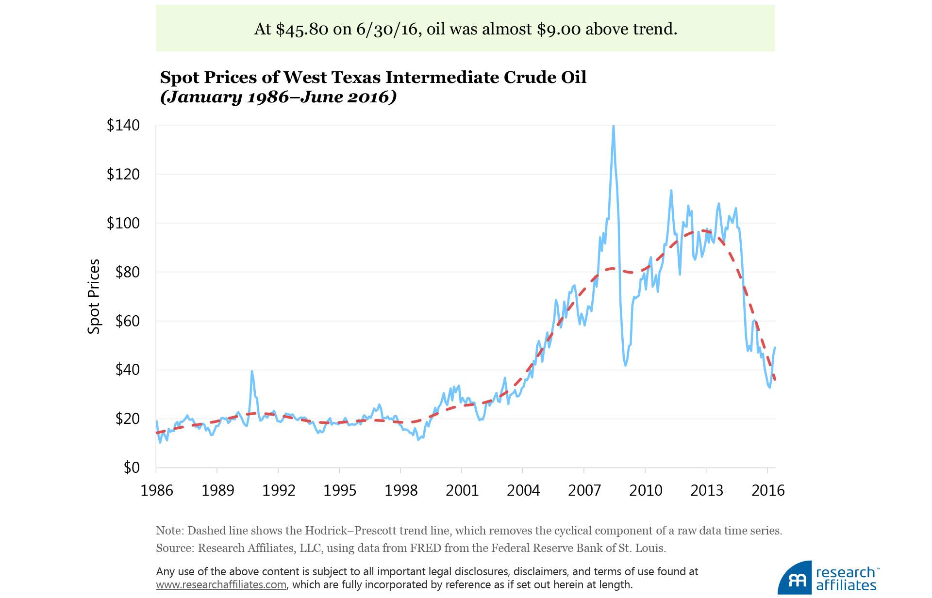
The trend in oil prices is heavily auto-correlated, so we can simply model the expected trend value in the subsequent period as the average return over the previous 12 months:

E[Trend Return_t+1] = Average (Trend Return_t,t-12)

Armed with this simple mechanism to describe the trend, the next step is to analyze the cyclical changes around it. Many of the factors influencing these changes do not stand out when we look at the full oil series, but become noticeable when we isolate the cyclical deviations from trend.

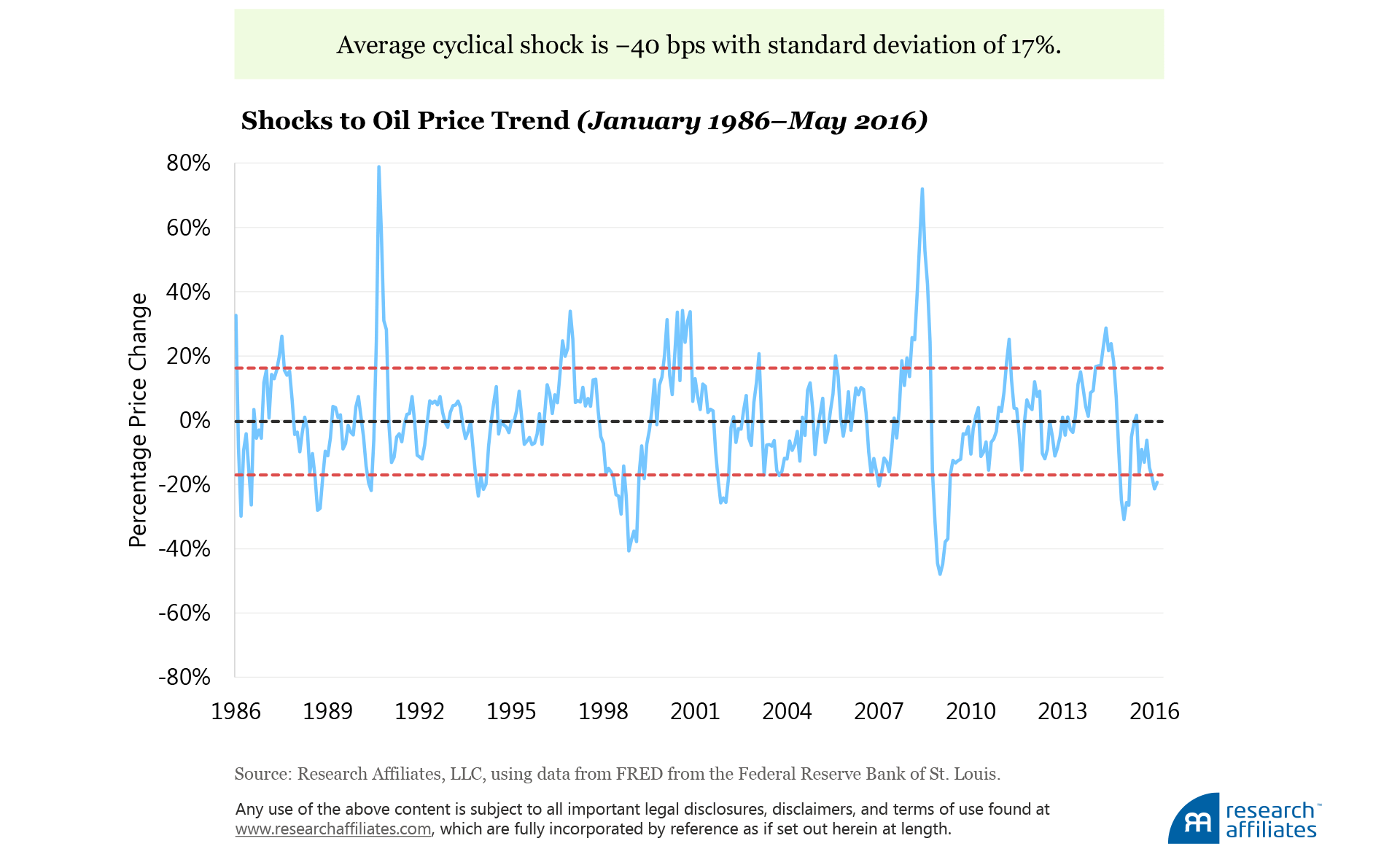
In the 30 years from January 1986 through June 2016, the average cyclical shock in the price of oil has been −40 basis points (bps) with a large standard deviation close to 17%. Negative shocks tend to be more prevalent (55% versus 45%) than positive shocks, whereas positive shocks have historically been larger in magnitude.

Oil shocks occur due to cyclical changes in the supply and demand drivers of the market. The four demand factors we use in our model are the 1) price return of copper, 2) value of the U.S. dollar relative to a basket of other currencies (DXY Index), 3) yield of the 10-year U.S. Treasury bond, and 4) slope of the oil futures term structure as specified by the two nearest-to-maturity contracts.

Copper’s return is a proxy for global growth, and therefore global demand, and thus captures the pace of global expansion. Because oil is priced globally in U.S. dollars, changes in the dollar’s strength affect the underlying price of the commodity for market participants whose preferred currency is not the dollar, such that the underlying economic value of the commodity remains unchanged. The 10-year U.S. Treasury yield is a proxy for the global risk appetite of investors; a lower yield suggests a lower risk appetite, leading to slower global growth and consumption. Finally, the slope of the oil futures term structure is a proxy for the estimated demand in the next period.

We use two supply variables: 1) U.S. oil production reported by the EIA and 2) monthly OPEC production reported by Bloomberg. These two factors are good examples of the types of variables that are masked if we analyze the return of oil as a whole, but become visible when we focus specifically on cyclical shocks.

The intuition is that shocks to these variables should drive shocks to oil prices around the otherwise slower-moving trend. Therefore, following the same process we use for oil, we can isolate the shocks from trend for each of the explanatory variables:

Oil Shock_t = Term Structure Slope_t + Copper Shock_t + USD Shock_t 
+ 10YR Treasury Shock_t + US Oil Production Shock_t + OPEC Production Shock_t

The only exception is for the slope of the futures term structure for which we use the simple difference between the prices of the second and first contracts. 

In adding the variables to the model, we have expectations about the sign of each. The signs of copper and the 10-Year U.S. Treasury bond are expected to be positive (and they are), which indicate times of higher global growth and of lower risk appetite, respectively. The signs of the U.S. dollar and U.S. oil production are expected to be negative (and they are), because a strengthening dollar should reduce demand for oil, and unexpected increases in U.S. production should provide greater supply for a given level of demand. The sign of the term-structure slope is also expected to be negative (and it is), because a positive slope indicates a term structure in contango, the situation in which spot prices are lower than prices of futures contracts, creating a negative roll return. Following are the coefficients from modeling oil shocks with the supply and demand factor shocks:

The positive coefficient on OPEC supply shocks could be viewed as surprising, but does make sense. As a supply variable, more OPEC production indicates greater supply and lower prices. OPEC, however, usually produces above trend only in environments when the market can support such production and prices are not expected to dramatically fall. This stance is consistent with the normal operation of a cartel, and not unexpected when analyzing data since the 1980s; this has definitely not been the case, however, over the last few years. To verify this intuition, an analysis of the relationship since 2014 shows the opposite (i.e., negative) sign on OPEC supply shocks.

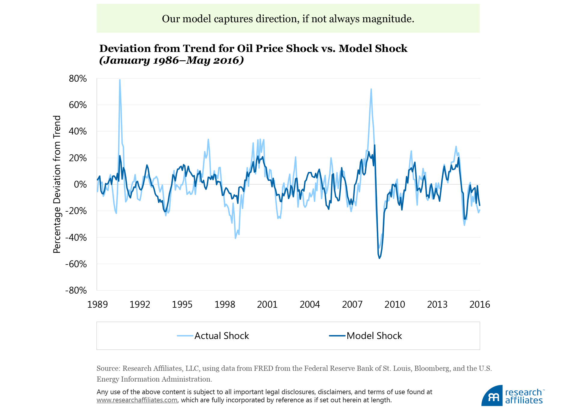
The time series results of modeling the shocks in oil prices by our set of supply and demand variables has an R² of 35.9%. Many of the directional changes in signal are modeled even though the magnitude of some of the larger deviations is only partially captured.

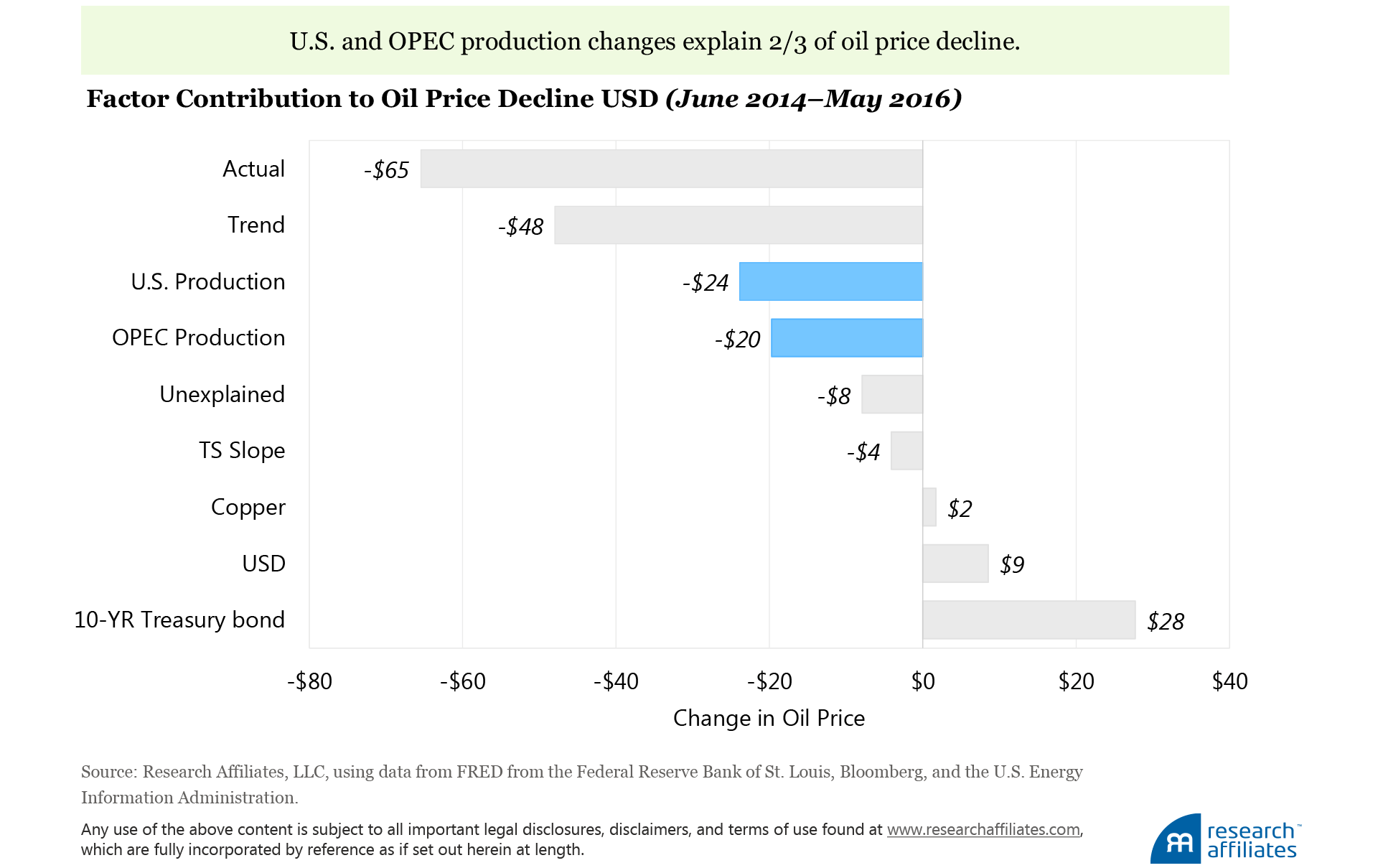
As we all know, oil prices have fallen more than 50% since their most recent peak just above $105 a barrel in June 2014. The decline has been attributed to a plethora of reasons, and using our model we can quantify which factors drove the decline. The recent increases in production by both the United States and OPEC were the most significant contributors to the drop in price, accounting for $44 of the roughly $65 total loss. Part of the loss was offset by an increase in bond yields (proxied by the yield of the 10-year Treasury bond), which indicates greater risk tolerance by investors. Because the model does not provide a perfect explanation for cyclical changes, an “unexplained” $8.00 accounts for the differences between modeled and actual changes in cyclical prices.

Philip Tetlock and Dan Gardner point out in their book, Superforecasting: The Art and Science of Prediction, that the attempt to derive a specific short-term forecast for the price of oil is “long a graveyard topic for forecasting reputations.” Not being speculators, we are—fortunately—unconcerned about estimating the price of oil in the next week or next month. Our primary interest is if oil prices a year from now will be in the $30–$50 range or return to the $100+ range, as these two scenarios have very different global ramifications for economic growth, inflation, and markets.

The historical period-by-period U.S. dollar contribution of each factor to the cyclical price of oil can help answer this question. Typically, a small cyclical variation from trend for each factor drives a small dollar change in the cyclical price of oil, however, wide differences do occur. Tail events can drastically alter oil prices, but are extremely rare.

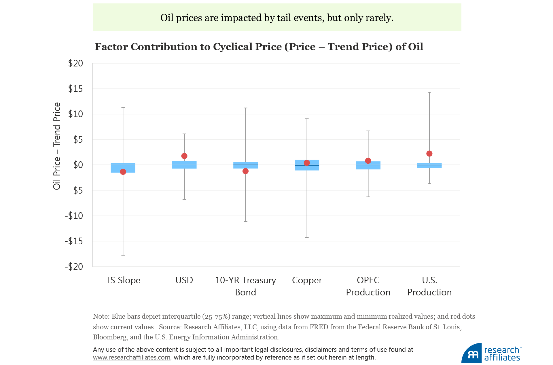
To evaluate the prospect of $100 oil, we create two simple scenarios based on the historical contribution from each factor. Modeling a trend price of $31.50 one year hence, we can create two scenarios: a realistic high-price case based on cyclical factors realizing their 75^th percentile change, and a much less realistic maximum-price case based on all factors hitting their historical maximum at the same time.

Under these two scenarios, our model produces a high-price expectation of $34.87, $11.00 below the price at the end of June, and a perfect storm maximum price of $90.12. Thus, even if all factors hit historical maximums, the price of oil is unlikely to hit $100 by summer 2017. The percentage change required by each factor to hit the maximum price and the high price vary considerably: 

Under the maximum-price scenario, the term structure slope would need to change from the current slope of $0.68 (contango) to a backwardated slope of $2.84, and the dollar must drop 12% from its current value. The high-price scenario involves much smaller changes from present levels, such as a 4% drop in the dollar.

To better understand the past and to get a sense of the likelihood of major changes in the future, we construct a simple model to decompose the trend in, and shocks to, the price of oil. The decomposition allows us to extract the underlying supply and demand factors that drive changes in the oil price. Our model, simple as it is, provides a mechanism for thinking about macro changes in oil prices and the changes in fundamentals necessary for large oil moves. Today our model indicates the price of oil at a one-year horizon (summer 2017) will remain similar in U.S. dollar terms to the current level. The implication for investors who are seeking greater diversification and higher yield than available in traditional asset classes is to allocate a portion of their portfolio to commodities, selecting those commodities not tilted heavily toward oil and oil-related products.

References

Bernanke, Ben. 2016. “The Relationship between Stocks and Oil Prices.” Ben Bernanke’s Blog, Brookings.edu, February 2.
Hamilton, James. 2014. "Oil Prices as an Indicator of Global Economic Conditions." Econbrowser.com, December 14.
Poghosyan, Tigran, and Heiko Hesse. 2009. "Oil Prices and Bank Profitability: Evidence from Major Oil-Exporting Countries in the Middle East and North Africa." IMF Working Paper 09/220, October.
Tetlock, Philip E., and Dan Gardner. 2015. Superforecasting: The Art and Science of Prediction. Crown Publishers: New York.
United States Energy Information Administration (U.S. EIA). 2016. “Short-Term Energy Outlook (STEO).” EIA.gov, July.