

Key Points
Trend-following strategies can offer attractive, positively skewed returns, with large positive outperformance often coinciding with large equity selloffs, thereby offering tail protection.
Not all trend strategies are the same. Increased positive skewness often comes with a lower Sharpe ratio, offering decision points for managers of such strategies.
The tradeoff between the Sharpe ratio and skew is directly related to signal and portfolio construction decisions.
Trend following is a simple strategy that takes long positions in assets that have been going up and short positions in assets that have been falling. With respect to equity markets, returns of trend-following strategies often show straddle-like returns, offering large positive returns when equity markets decline and more modest returns in up markets. Although trend following has reached broad popularity among investors only over the past decade or two, Hurst et al. (2017) shows that the benefits of trend following have existed for over a century.
Trend following has a return pattern in which positive skew tends to coincide with equity drawdowns, which makes this strategy ideal for many portfolios. In fact, from the perspective of high-level asset allocation, one may consider a portfolio in terms of four pillars: economic growth, income defensiveness, alpha, and tail protection. One straightforward approach is to populate these pillars with investments in equities (economic growth), bonds (income defensiveness), absolute-return strategies (alpha1), and trend following (tail protection).
Trend following has a return pattern in which positive skew tends to coincide with equity drawdowns, which makes this strategy ideal for many portfolios.
In other words, trend-following strategies require investors to perform a delicate balancing act, walking the tightrope between risk-adjusted returns (Sharpe ratio) and tail protection (positive or negative skew). Maximizing one comes at the cost of diminishing the other, which may put a portfolio out of balance with a desired objective. As this article illustrates, understanding the nuances of the relationship between Sharpe ratio and skew can enable investors to make wiser decisions about portfolio construction, ideally leading to their optimal tradeoff.
At its core, the construction of trend-following strategies is a trade-off between Sharpe ratio (i.e., higher average risk-adjusted returns over time) and positive skewness. The tail protection comes from the skew, but the Sharpe ratio should not be overlooked because it is often what allows investors to remain in a strategy during extended bull markets.
The tail protection comes from the skew, but the Sharpe ratio should not be overlooked because it is often what allows investors to remain in a strategy during extended bull markets.
This tradeoff has been harder to maintain over time. To illustrate this point, Figure 1 uses the SG Trend Index (an aggregate of the performance of large trend-following strategies) as a proxy. From the first part of the century to the most recent 10 years, the average return for these trend strategies dropped by almost half.
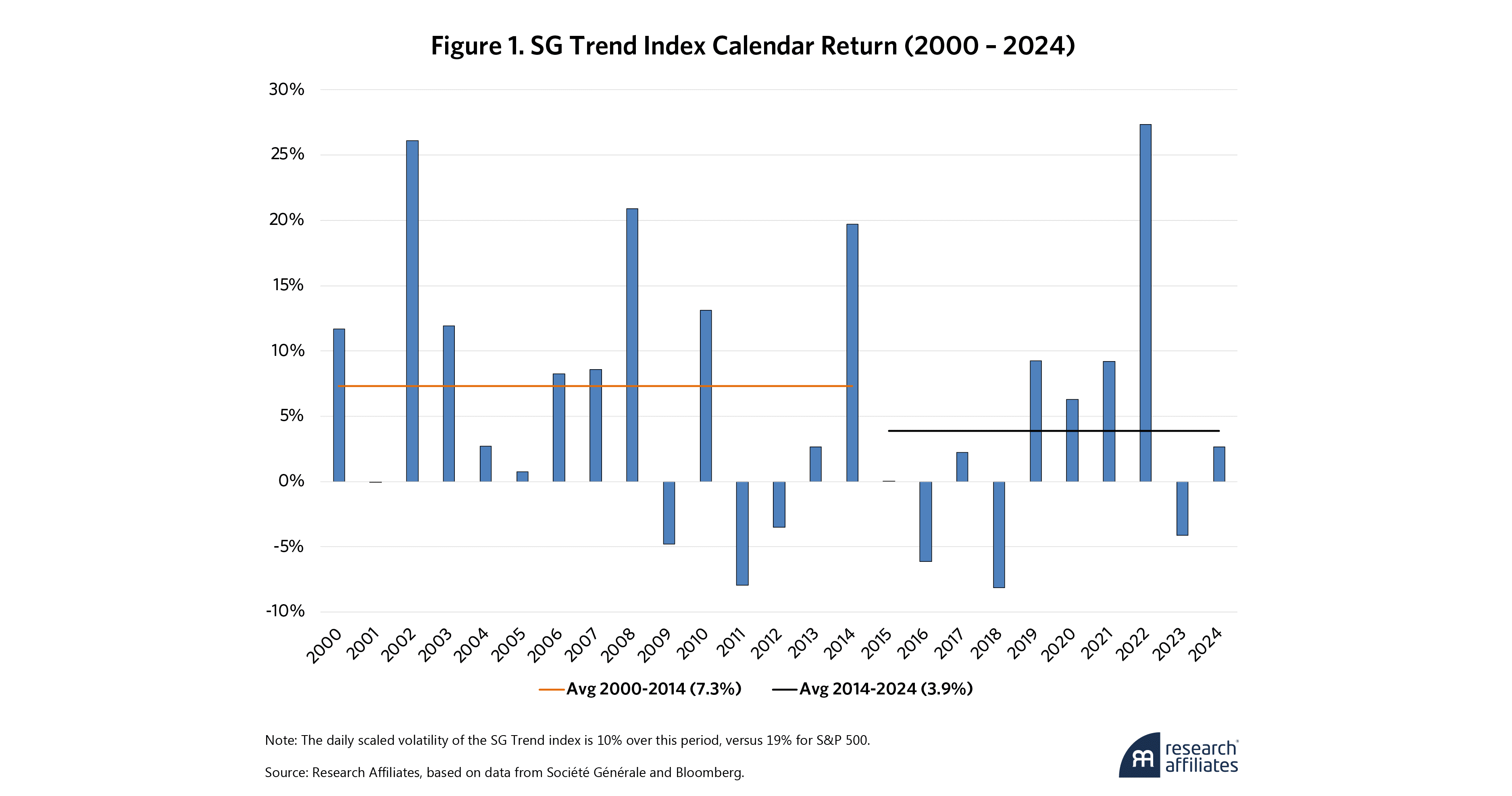
During good times, investors often forget why they bought the policy in the first place. In other words, they forget why they are allocating to a lower-returning trend portfolio instead of the other parts of the portfolio that are offering higher returns. According to Greyserman (2017), “Trend following’s positive skew creates a tension with the Sharpe ratio, as investors may misjudge performance due to behavioral biases favoring frequent small wins over rare large gains.” In other words, trend is like an insurance policy: investors pay premiums in the form of many small losses during periods of low volatility in exchange for winning big in a high-volatility event.
The SG Trend Index also can be used to illustrate the trend tradeoff between Sharpe ratio and skew, as shown in Figure 2. For both short (2-year) and longer (5-year) time horizons, the relationship between Sharpe ratio and skew has a negative slope.
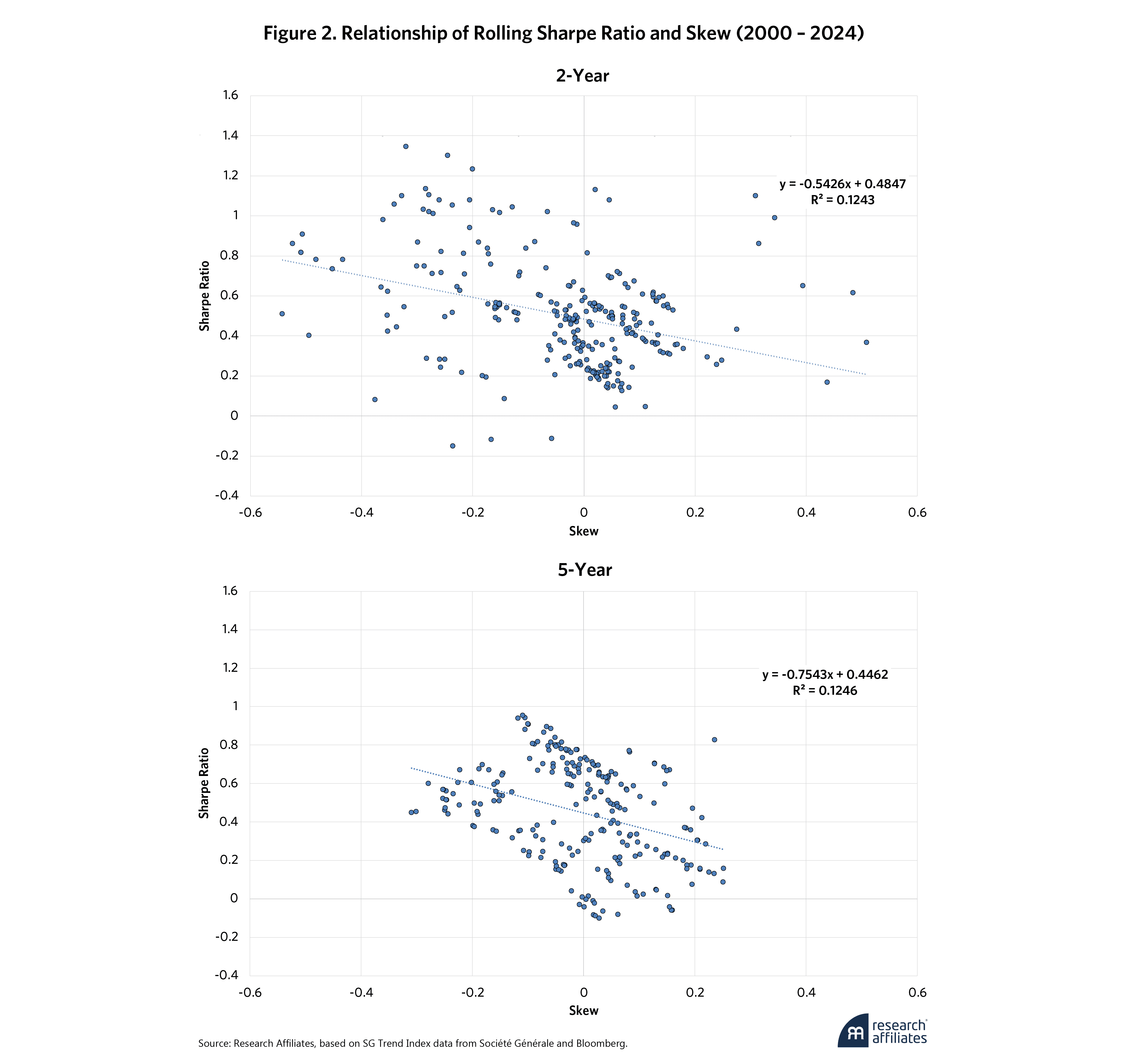
This relationship is important because the large positive returns that drive the positive skew often coincide with drawdowns in the equity market. For example, for the S&P 500’s three worst calendar years since the start of the century, as shown in Table 1, the SG Trend Index had positive double-digit returns in all three years, generating annual outperformance of close to 50%.

When considering adding a trend mandate to portfolios, investors need to understand that not every trend portfolio is the same. It’s also critical to consider the characteristics of the particular trend strategy and whether the strategy meets the objectives for putting it in the portfolio in the first place. As mentioned above, tail protection can be a key pillar in the design of a portfolio, but even so, that is not to say that every investor should focus exclusively on the most positively skewed portfolio at the expense of the overall Sharpe ratio. A better tradeoff solution often can be found. To help investors understand how the tradeoff works and its implications, this article looks at a few of the key portfolio construction decisions that face trend managers and their tricky tradeoffs.
Sharpe Ratio and Skew
The calculation of the Sharpe ratio is familiar to most professional investors.2 Skew, however, is a different matter. Although skew is often discussed, many investors don’t actually think about its interpretation or how it is calculated:
Sample skew is calculated as the cubic difference in return from average over the entire period divided by the cubic standard deviation over the period.3 For return series with the same return dispersion, skew is directly proportional to the inverse of cubic volatility (with squared volatility being the variance).
Visual representations are often the easiest way to internalize the difference in skew values, as shown in Figure 3. Distributions with skew values close to zero are symmetrical in nature, including the normal and uniform distributions. As the skew rises, the distribution will exhibit more and more outliers in one direction or the other. This pattern is one of the challenges with measuring skew and is responsible for why skew is often described as being unstable. By definition, skew means trying to measure observations in the tail of distribution where fewer observations exist.
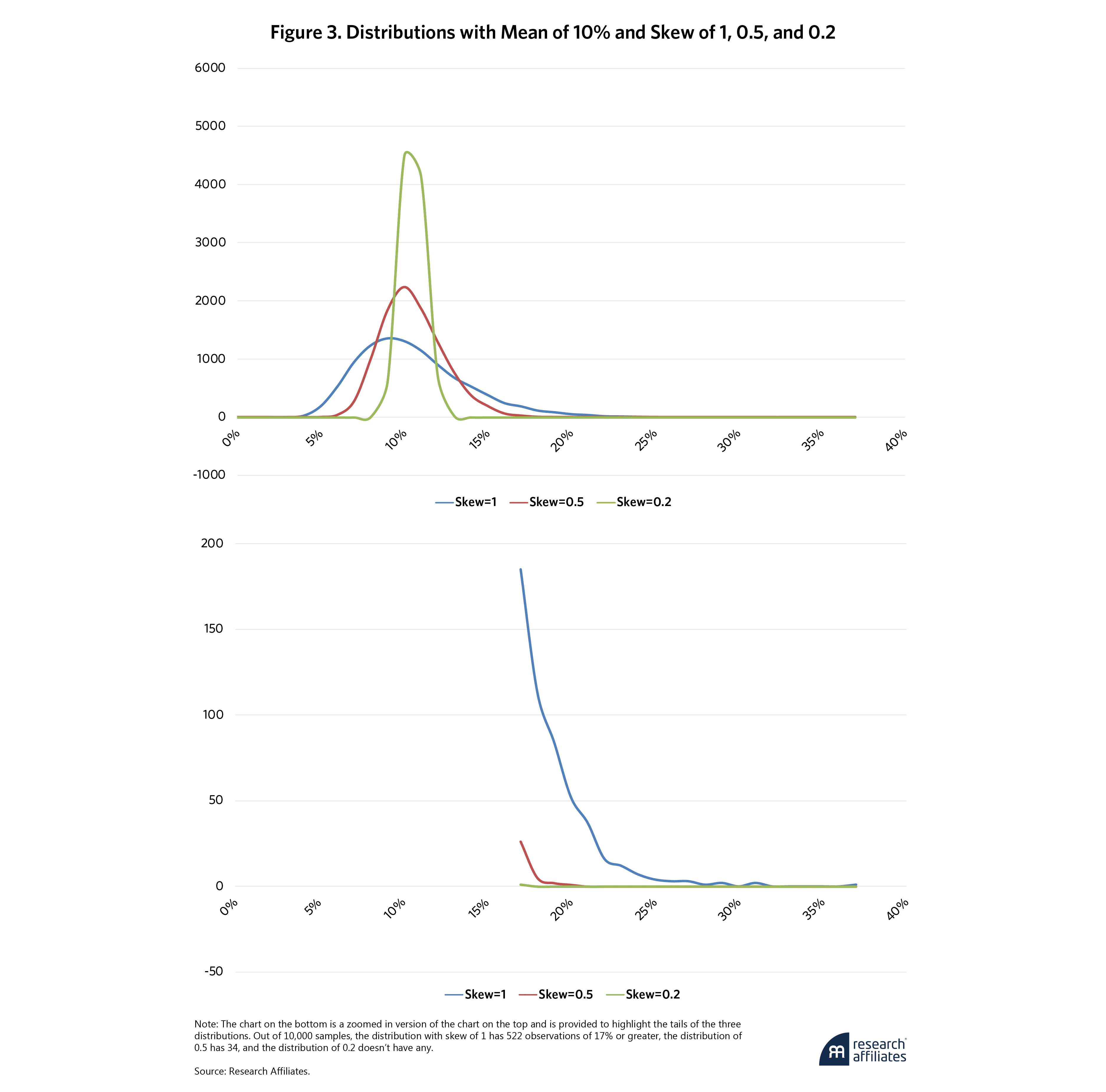
Skew is also indifferent to scaling. Because ex-post volatility scaling of a series of returns will not adjust the skew, the skew can be compared across assets or strategies with different volatilities.
Finally, although various methods have been proposed to adjust the estimation of Sharpe ratio to incorporate skew, with two examples being Maillard (2018) and Bailey and de Prado (2012), this article uses the standard Sharpe ratio estimation method because it is most familiar to and broadly used by practitioners.
Data
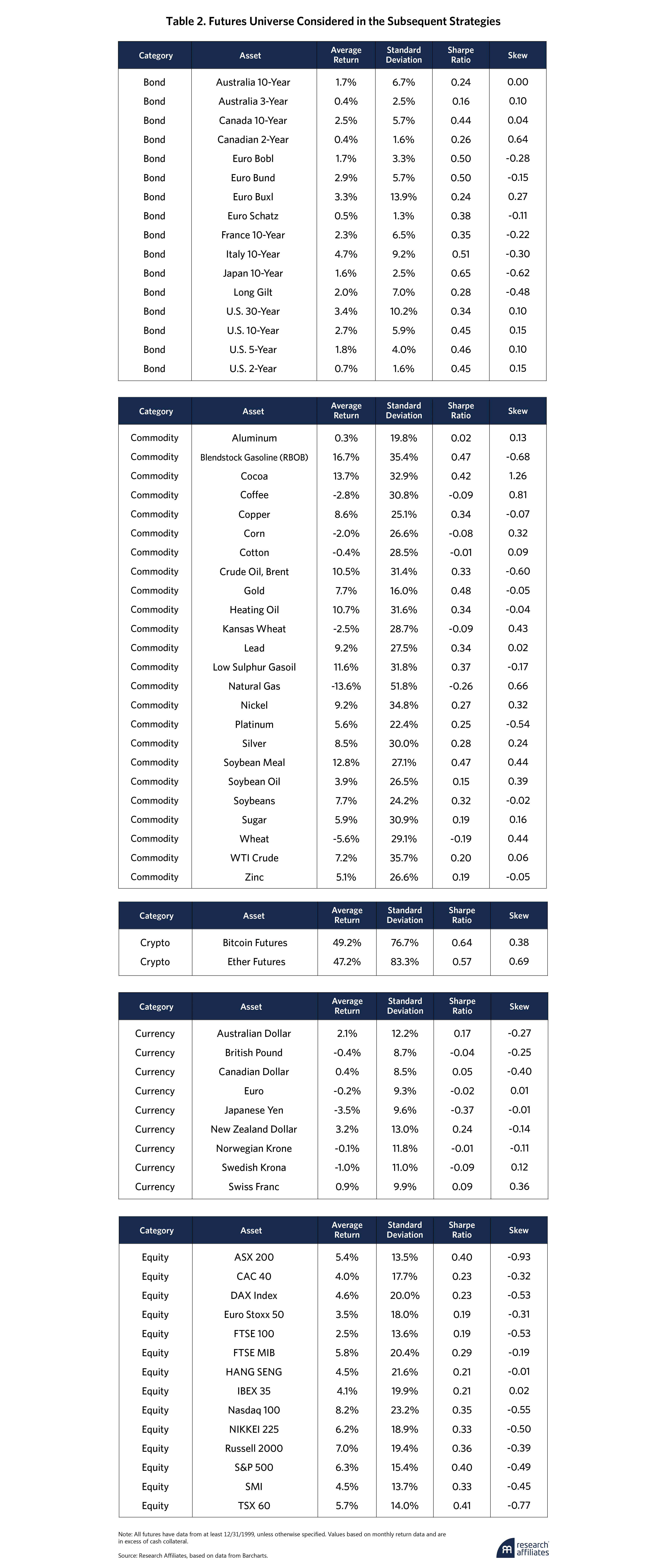
In order to analyze the tradeoff of Sharpe ratio and skew in trend following, we create a trend strategy using a universe of 65 futures across equities, bonds, currencies, commodities, and cryptocurrencies. This universe, shown in Table 2, is by no means exhaustive of all liquid futures used by trend managers, but it provides a broad cross-section of exposures that exist in most commercial trend portfolios.
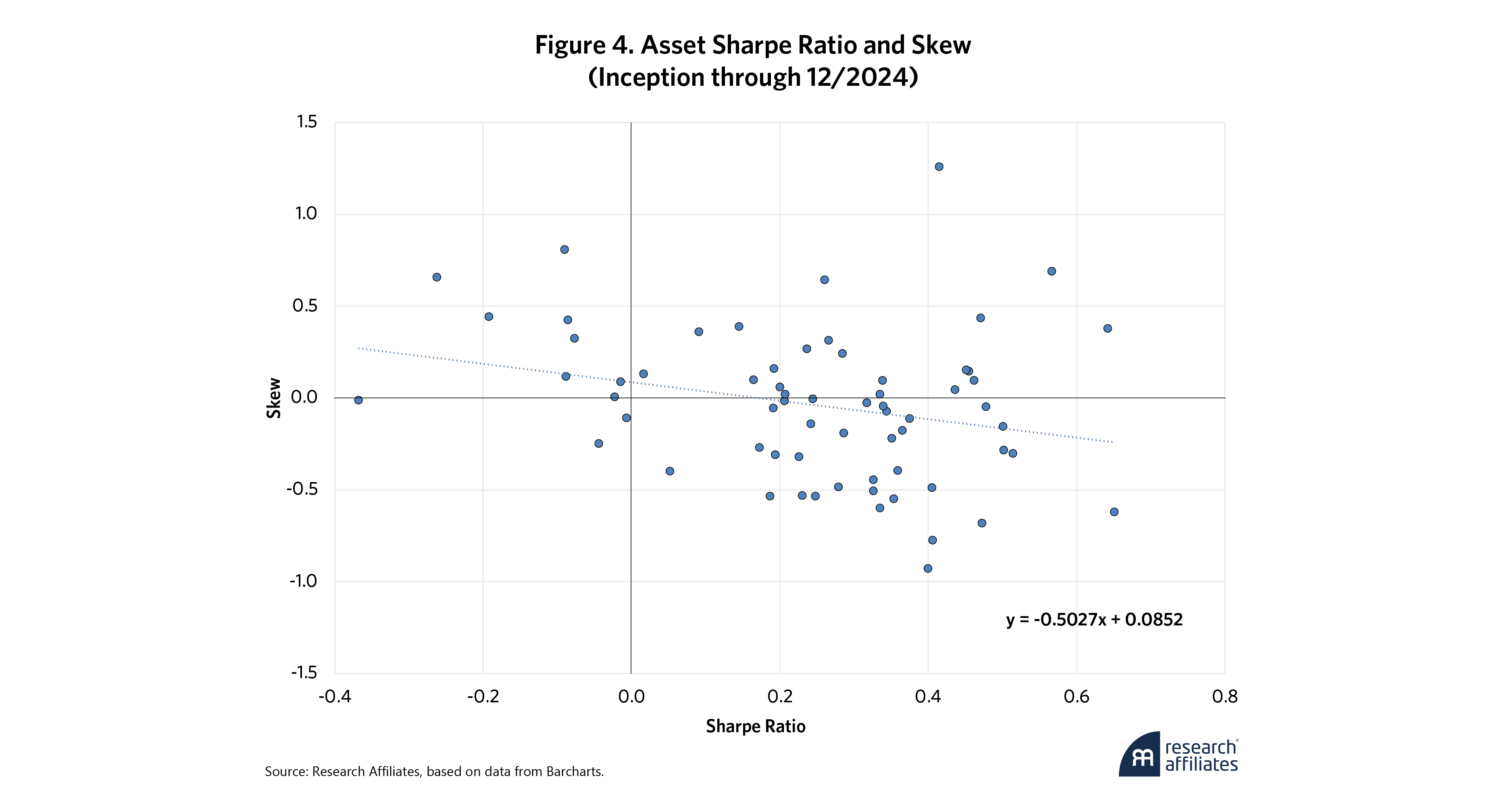
At an asset level, to better visualize the relationship between Sharpe ratio and skew, we plot these values for the entire universe of assets, as shown in Figure 4. As discussed, this shows a negative relationship, with lower Sharpe ratio assets having higher skew, and vice versa, but with a few notable outliers. In a similar finding, Harvey and Siddique (2000) note the negative relationship between expected returns and skewness across equity securities.
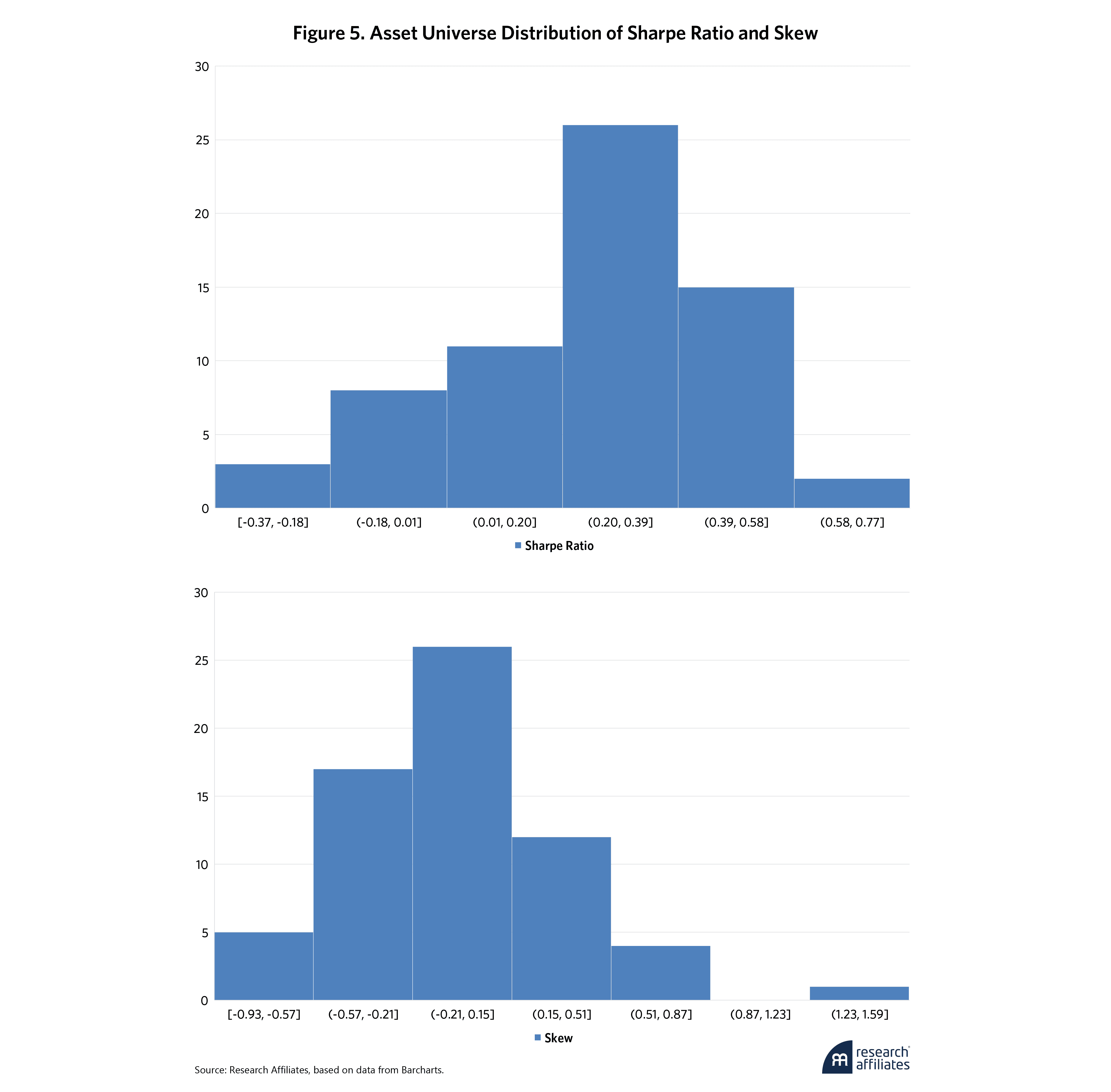
The average Sharpe Ratio for this universe of assets is 0.25, with a negatively skewed distribution, as shown in Figure 5. The average skew across this universe of assets is close to zero, but with a few positive outliers, such as cocoa.
Trend Portfolio Construction
To illustrate the trade-off between Sharpe ratio and skew in a trend-following strategy, we construct portfolios using a simple signal—exponentially weighted moving-average crossover (MAC)—to measure assets’ trends.4 This signal considers two lookback periods: fast and slow, which identify the half-lives of each moving average. If the moving average price of the fast lookback is above that of the slow lookback, a long position is taken. When the fast lookback price is below the slow lookback price, a short position is taken. For example, if the fast-period average price was $100 and the slow-period average price was $98, we would take a long position in the asset. For those readers more comfortable with time-series momentum, Levine and Pedersen (2015) show that the moving-average crossovers and time-series momentum are closely related.
Even though we are using a relatively simple signal to construct our portfolio, there are still a number of portfolio construction decision points that impact the trade-off between Sharpe ratio and skew. More sophisticated strategies will have even more decision points. For the purpose of this article, we consider four such decisions:
Half-life Lookback: The length of the half-life for each of the exponentially weighted moving averages used to measure the trend. For MAC, this means the slow and fast windows.
Weight Response Function: The size of the position in the trend portfolio can be based on the sign of the trend or on the magnitude of the trend. With the sign-based approach, the weight of each asset will be based on the volatility of the asset to give an equal risk contribution regardless of the strength of the trend signal itself. With the magnitude approach, the weight of the asset in the portfolio will be directly related to the strength of the trend signal through a mapping. In this article, we map the magnitudes to weights through a simple sigmoid5 function.
Asset Volatility: As with many trend managers, we choose to equal volatility-weight the positions in the portfolio with the objective of having equal risk contribution. The window used to measure the volatility impacts the tradeoff.
Portfolio Volatility: To capture the benefits of many trend configurations, a final trend strategy is often the combination of a number of underlying strategies with various parameters. As with assets, we choose to focus on equal volatility weighting across the strategies, and the window used to measure the volatility impacts the tradeoff.
The following sections step through each of these decisions one by one to illustrate the impact and tradeoffs in a broad set of configurations.
Tradeoff 1: Trend Signal Half-Life Lookback
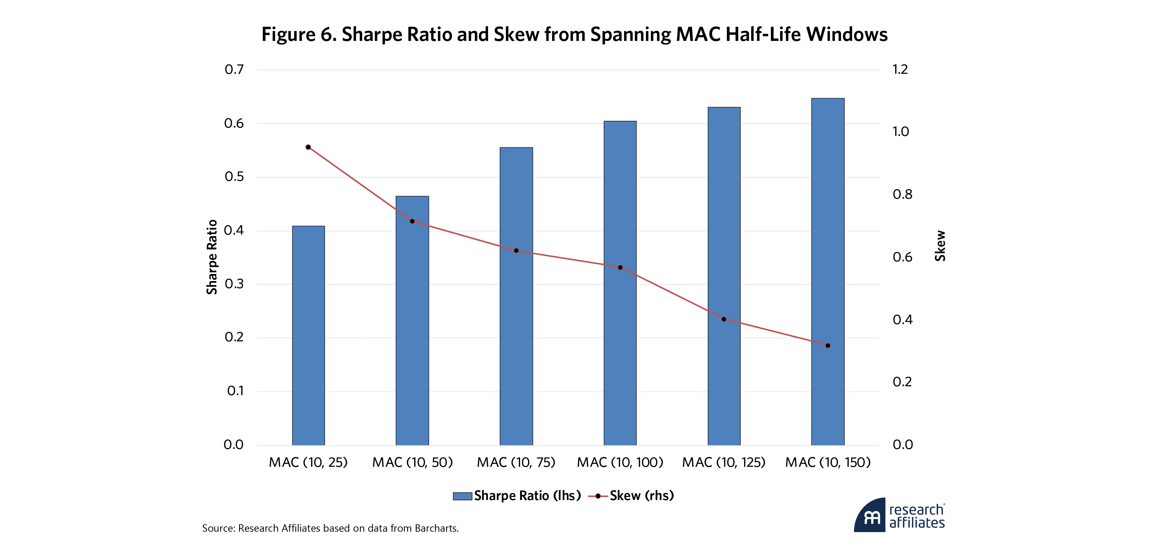
Starting simple, we first look at altering the half-life of the slow lookback signal of the moving average crossover (MAC), keeping the fast signal constant at 10 days. As shown in Figure 6, the slow half-life starts at 25 days and increases to 150 days in increments of 25 days. Even in this simple configuration, we see the Sharpe ratio of the “fastest” configuration (10-days, 25-days) has the lowest Sharpe ratio at 0.41 and the largest positive skew at 0.95. As the half-life lengthens, the Sharpe ratio monotonically increases while the skew monotonically falls. This finding is not specific to the MAC signal, for example, Mackic (2023) shows similar results using a double exponentially weighted moving average crossover signal.
As previously mentioned, positive skew often accompanies extreme selloffs in equity markets. For example, consider the first quarter of 2020, when the world was first coming to grips with the spread of COVID-19. Markets had steep selloffs that started in mid-February and continued through early April. As Table 3 shows (not unexpectedly), faster response functions were able to quickly pivot and achieve positive returns while the slower signals struggled to keep up, although the slower signals still outperformed many other classes.

Tradeoff 2: Signal to Weight Response Function (Sign vs. Magnitude)
For creating a trend portfolio, two common rules are (1) to weight all assets based on the sign of the trend signal (positive/negative sign rule) or (2) to weight assets based on the magnitude of the trend signal. Although many functions can be used to map the trend signal to a weight, we use a simple sigmoid function to illustrate the impact of response-function choice on the tradeoff of Sharpe ratio and skew.6
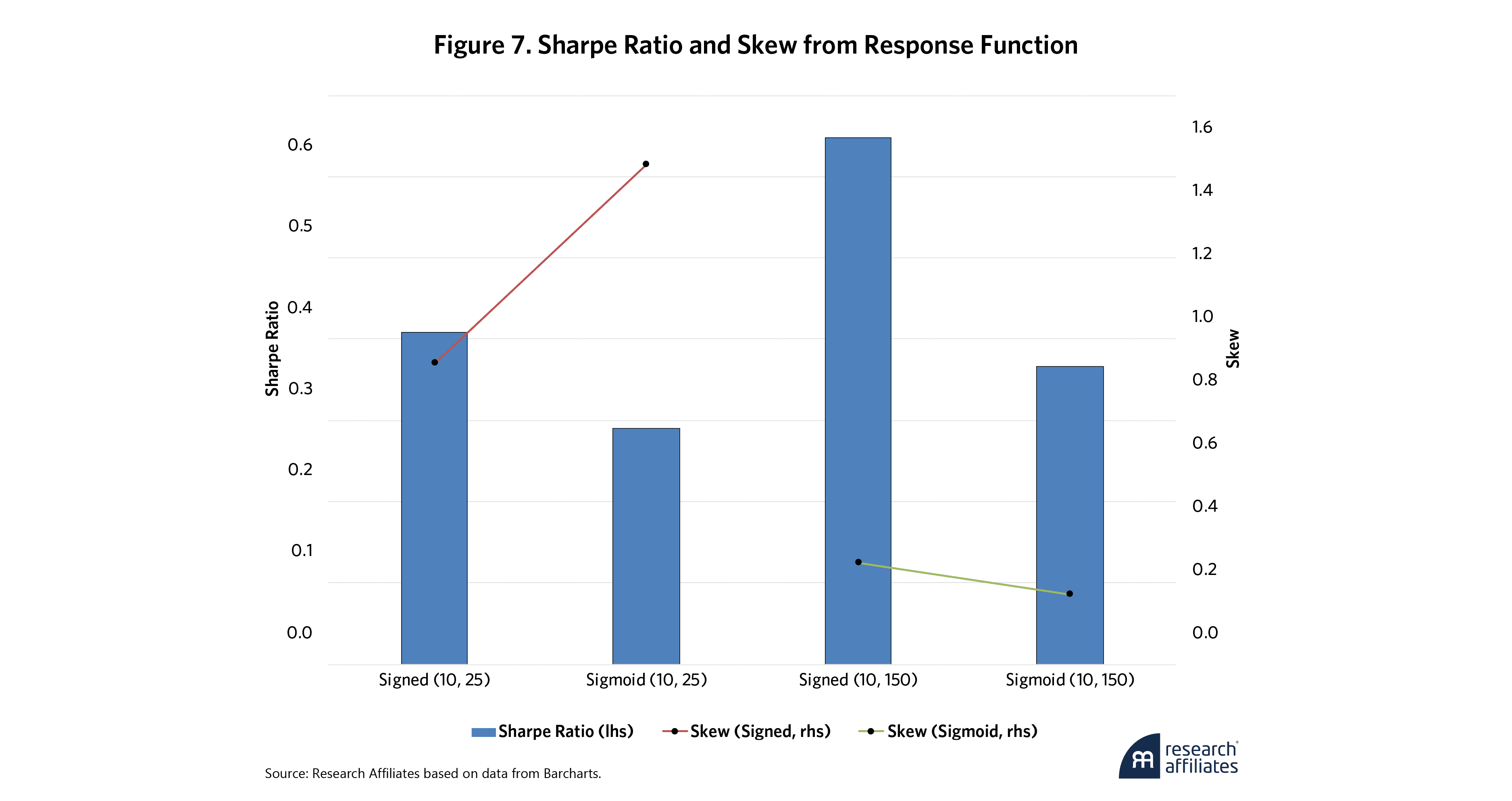
To compare response-function impact, it’s also helpful to view multiple lookback half-life windows as described for tradeoff 1, as shown in Figure 7. For short-lookback windows with fast response, the sigmoid function has a lower Sharpe ratio but a much higher positive skew than the signed response function. This finding implies that the sigmoid approach is able to benefit greatly from taking large positions in assets that have shown meaningful quick dislocations in price from their trend. But to get a few large winners, the tradeoff is also to get a number of losers, which impacts the overall Sharpe ratio of this approach.
To get a few large winners, the tradeoff is also to get a number of losers, which impacts the overall Sharpe ratio of this approach.
Interestingly, with the longer window, the signed response function maintains its Sharpe ratio advantage over the sigmoid, but the difference in skew is minimal. More importantly, however, the positive skew of both functions is getting closer to zero.
October 2008 is a well-known outperformance month for trend strategies. In our simulations, aggregate energy (oil, gas, etc.) provides an example of the power of weighting by trend strength. Its weight in the sigmoid portfolio was –11% (short position) versus a weight of –3% in the equal volatility-weighted sign portfolios.7 In October 2008, energy futures were down almost 30% on average.
Tradeoff 3: Asset Volatility Weighting in Sign-Based Portfolios
As noted above, the signed response function only considers the direction (positive or negative) of the trend signal. The method to convert the sign of the trend to a weight is often based on the asset’s volatility. This method (equal volatility weighting) attempts to weight assets such that they have the same risk contribution to the portfolio.
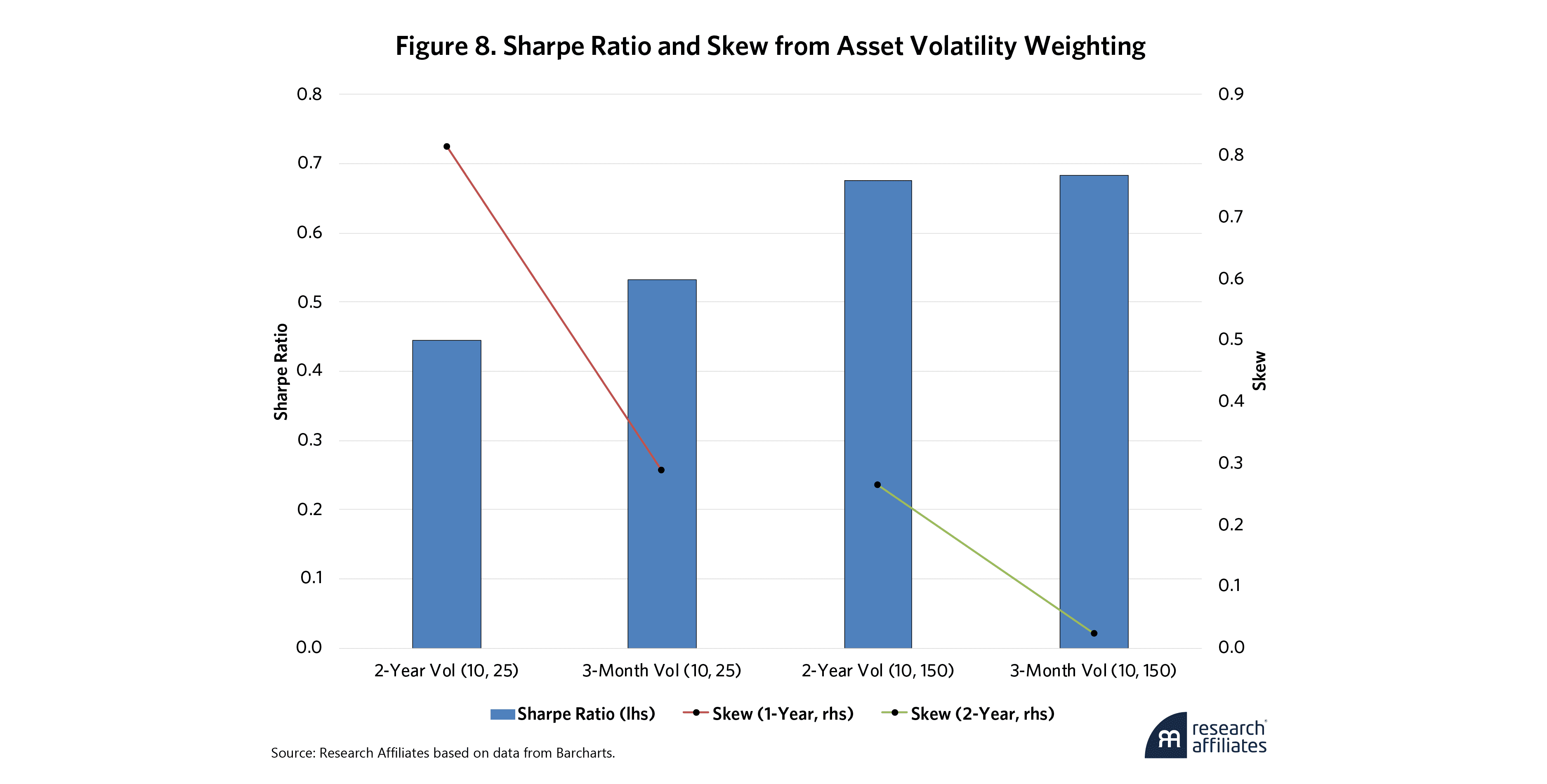
How the assets’ volatilities are measured can also have an impact on the tradeoff of Sharpe ratio and skew. To demonstrate, Figure 8 shows two different lookback half-lives: (10, 25) and (10, 150). Unlike the lookback half-life, where the shorter lookback had higher skew, the opposite occurs with measuring the asset’s volatility. The same relationship holds for the longer lookback, but another important aspect is that a longer lookback tied to a short asset volatility window (3 months) all but negates any positive skew in the portfolio. In contrast, a shorter lookback with a longer asset volatility window (2 years) has a positive skew of approximately 0.8.
The reason for this tradeoff may be self-evident. Trend following is a long volatility strategy. Short measures of volatility (e.g., 3 months) will be more volatile than will long measures. When volatility rises in the short term, the short measures will rise more than the long measures, causing the weight in the asset to fall. This pattern is in direct opposition to the desired effect of a trend strategy, which should lean into volatility when it rises.
Tradeoff 4: Trend Strategy Volatility Weighting
Finally, trend mandates often combine many underlying trend portfolios that span some of the previously mentioned parameters. To demonstrate, we average the 12 portfolios (six signed and six sigmoid portfolios across lookback windows) using an equal volatility approach.8 The tradeoff in this case, is the window used to measure the volatility of the 12 portfolios in order to determine the weight of each one, as shown in Figure 9.
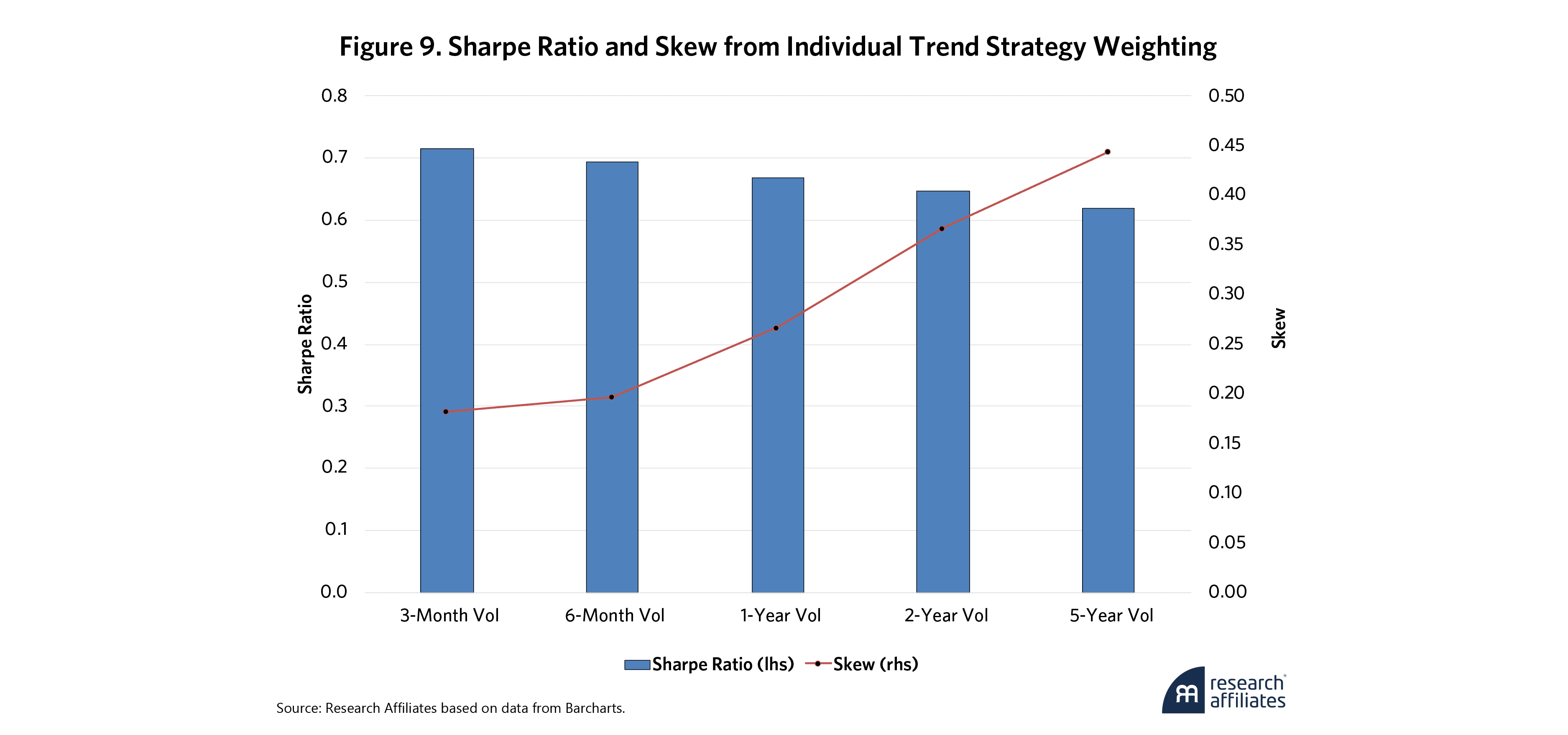
Averaging portfolios in this way is advantageous because one only needs to give up some moderate Sharpe ratio to double the positive skew. To better illustrate these results, consider only the 3-month volatility window and the 5-year window. The 3-month window will obviously be more responsive to changes in market conditions, causing the volatility of each portfolio to be higher when markets are more volatile. In contrast, the 5-year window will move more slowly.
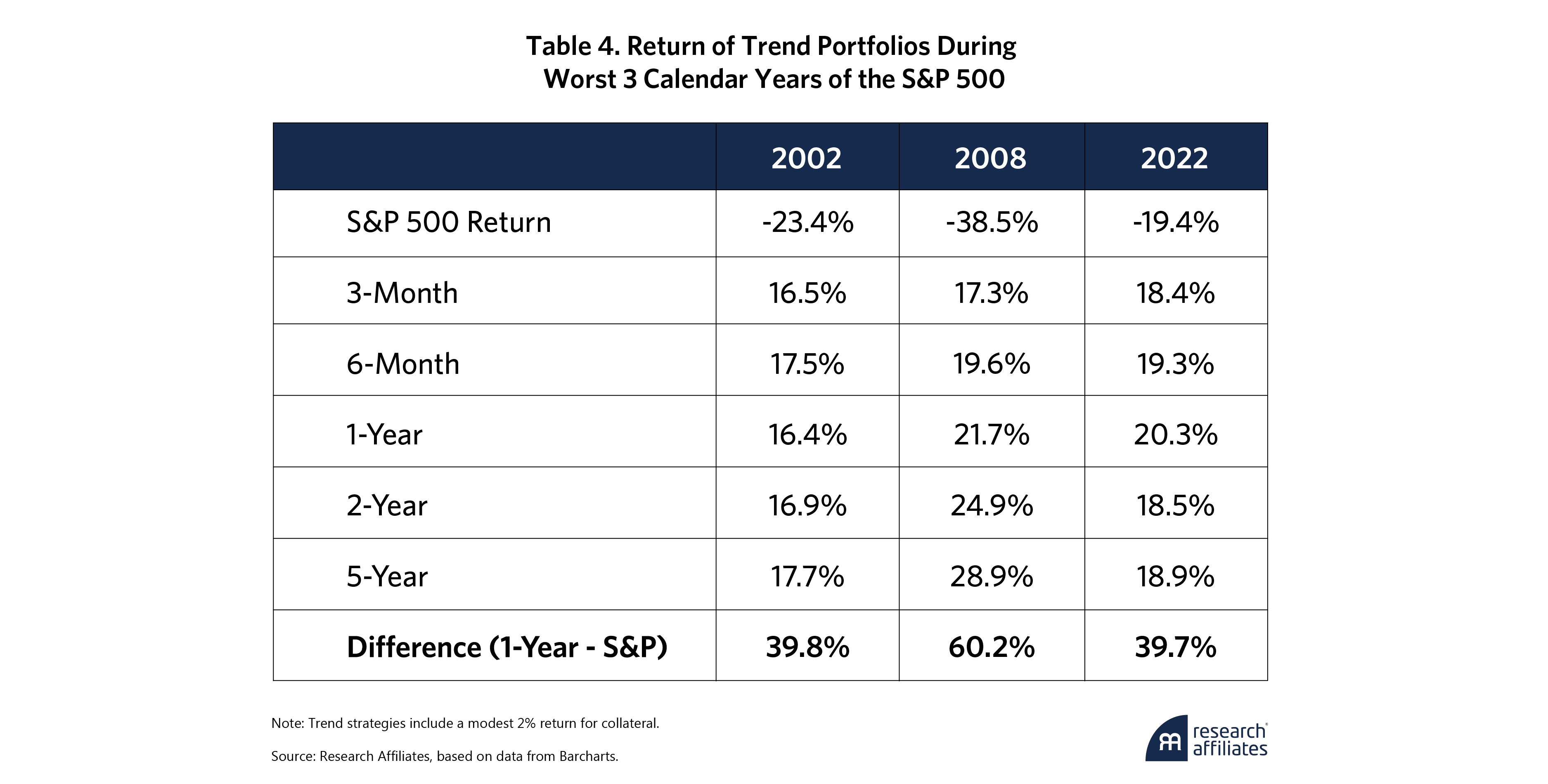
Finally, Table 4 compares each of these portfolios to the S&P 500 during the three years when the S&P 500 had large drawdowns and SG Trend Index far outperformed. Although the highest-skew portfolio (5-year) was best in 2002 and 2008, it underperformed a bit in 2022. This difference highlights the fact that a trend strategy that combines underlying strategies with various parameters can provide investors with a nice tricky tradeoff in the Sharpe ratio–skew negotiation.
Conclusion
Much like a balance pole for a highwire act, trend-following strategies provide an important and subtle tool for portfolio construction, but to wield it deftly, investors need knowledge and skill. Clearly, trading Sharpe ratio for positive skewness can provide valuable portfolio protection during market downturns, and as this article has explained, four key portfolio construction decisions impact this tradeoff:
Trend-signal half-life lookback
Signal-to-weight response function
Asset volatility weighting
Trend-strategy volatility weighting
Each of these decisions presents opportunities to fine-tune the balance between consistent performance (Sharpe ratio) and tail-risk protection (positive skew). The analysis demonstrates four key findings:
Shorter lookback periods tend to increase skewness at the expense of Sharpe ratio.
Sigmoid response functions can enhance skewness, particularly for shorter lookback windows.
Longer asset volatility measurement windows can preserve positive skew, especially for shorter trend lookbacks.
Combining multiple trend strategies with appropriate volatility weighting can optimize the Sharpe ratio–skew tradeoff.
Ultimately, the ideal configuration depends on an investor's specific objectives and risk tolerance. While maximizing positive skew can provide superior protection during severe market downturns, it may come at the cost of lower overall risk-adjusted returns during calmer periods. At Research Affiliates, we generally lean towards trading off Sharpe Ratio for more positive skew.
While maximizing positive skew can provide superior protection during severe market downturns, it may come at the cost of lower overall risk-adjusted returns during calmer periods.
By understanding these tradeoffs, we hope investors can make informed decisions about how to implement or identify trend-following strategies that align with their long-term goals and risk management needs.
End Notes
1. With respect to core stock and bond (i.e., core beta) exposures.
2. For those needing a refresher, Sharpe ratio is the excess return of the strategy relative to the risk-free rate divided by the volatility of the strategy:
3. Here we focus on the standard measurement of sample skew, but many other formulations exist.
4. In this article, we ignore the impact of transaction costs. In addition to simplicity, the higher-turnover (transaction cost) portfolios already have a lower Sharpe ratio. Including transaction costs would therefore just reinforce the findings.
5. A sigmoid is an S-shaped function in which small trend magnitudes get small weights. As the magnitude of the trend increases, so does the weight, and this process continues at an ever-increasing rate until a high-water mark is reached, at which point the rate of change of the weight with respect to the signal change is reduced.
6. For a detailed discussion of various response functions, see Martin (2023).
7. These exposures have been normalized to a 100% gross leverage portfolio.
8. The choice to equal volatility-weight the sigmoid portfolios was done for simplicity of this example and may not be the optimal weighting scheme.
References
Bailey, D. H., M. López de Prado. 2012. “The Sharpe Ratio Efficient Frontier.” Journal of Risk 15(2): 3–44.
Greyserman, A., K. Kaminski, A. Rudin. 2017. “Skewness and Trend Following: A Behavioral Perspective.” Journal of Alternative Investments 20(2): 7–19[1].
Harvey, C. R., A. Siddique. 2000. “Conditional Skewness in Asset Pricing Tests.” The Journal of Finance 55(3): 1263–1295.
Hurst, B., Y.H. Ooi, and L.H. Pedersen. 2017. “A Century of Evidence on Trend-Following Investing.” The Journal of Portfolio Management 44(1): 15–29.
Levine, Ari, and Lasse Heje Pedersen. 2015. "Which Trend Is Your Friend?" Journal of Financial Economics 115(1) 5–33.
Mackic, A. January 2023. “The Need for Speed in Trend-Following Strategies.” Man Group.
Maillard, Didier. 2018. “Adjusted Sharpe Ratio: Some Caveats.” SSRN Working Paper 3284396.
Richard J. Martin. 2021 (revised Jan 2023). "Design and analysis of momentum trading strategies." Papers 2101.01006, arXiv.org.