
Rather than predicting what will happen to inflation in the future—a particularly arduous and humbling task—we ask a simple question: What can past inflation dynamics tell us about the equity market’s future returns?
We propose two new investment signals, which we label inflation cycles and surprises, and document that negative cycles and surprises predict higher equity returns in excess of the risk-free rate. We employ this predictability to design a new market-timing strategy: buy equities when inflation cycles and surprises are negative, and sell them otherwise.
We show that the predictability of cycles and surprises varies across equity sectors. We exploit these differences in predictability to design a novel sector-rotating strategy.
We highlight how inflation signals have worked consistently well across decades in addition to inflation and market regimes. Unlike commodities, tactical strategies based on inflation signals appear to perform well during both positive and negative market environments.
Conversations in the investment industry have been dominated by predictions about the path of the inflation rate and its implications for capital markets. In this article, we aim to turn these conversations upside-down. We propose two new investment signals, which we call inflation cycles and inflation surprises. We find that negative cycles and surprises predict higher equity returns in excess of the risk-free rate, and we use this predictability to design a new market-timing strategy that buys equities when inflation cycles and surprises are negative, and sells them otherwise. We also show that the predictability of these signals varies across equity sectors and exploit these differences to design a novel sector-rotating strategy.
Create your free account or log in to keep reading.
Register or Log in
Why Inflation Dynamics Should Predict Risk Premia
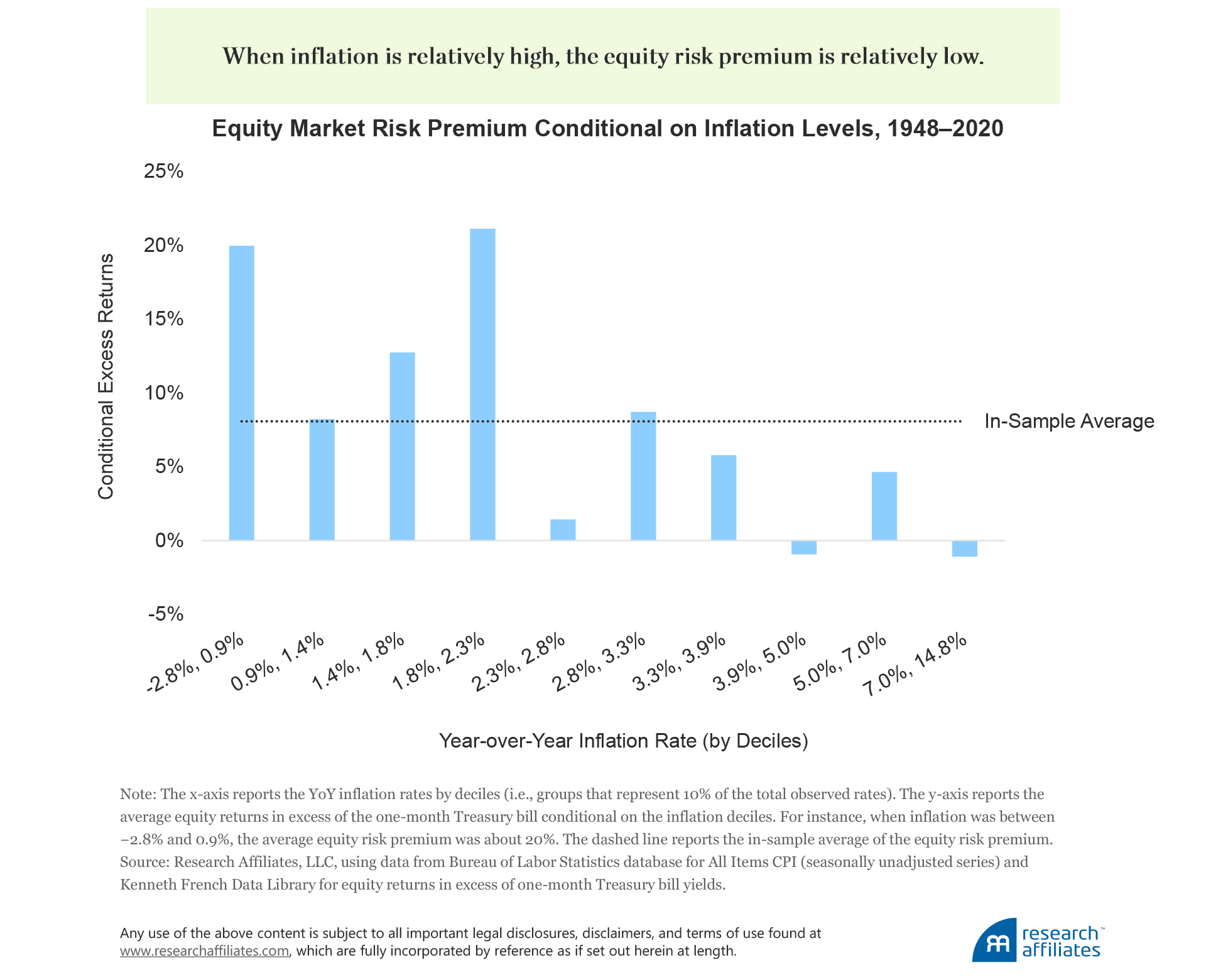
Multiple articles document that equity markets tend to underperform when inflation is relatively high.1 To appreciate this relationship, we examine the average excess returns of the US stock market conditional on the contemporaneous year-over-year (YoY) inflation level for the period January 1948–December 2020. We find that when inflation is relatively high, the equity risk premium is relatively low, and is a statistically significant relationship. Unsurprisingly, today’s renewed inflation fears are dominating conversations in the investment industry. The determination of governments and central banks to provide support to their economies is leaving investors wondering whether prices may spiral as they did in the 1970s when inflation reached double digits.
The negative relationship between inflation rates and the equity risk premium may be unexpected to some because equities are a claim on real assets and, therefore, should provide a hedge against inflation. Fama (1981) offers an explanation for this evidence, noting that inflation may be a proxy for the business cycle and that periods of high inflation can coincide with periods of subdued real activity (i.e., stagflation). Related to this argument, Bekaert and Wang (2010) note that the discount rate channel likely plays a major role because risk premia increase during recessions (i.e., investors become more risk averse). We build and expand on these arguments by leveraging the Phillips Curve, a key concept in economics that classically relates inflation to unemployment.
In its modern version, the Phillips Curve is a reduced-form equation that connects the current inflation rate to inflation expectations and the business cycle. By approximating inflation expectations with an average of past inflation rates, we can generalize the Phillips Curve as follows:
Current Inflation Rate \(\cong \) Average of Past Inflation Rates + Output Gap
The Phillips Curve makes a simple point: Firms will react to changing expected costs of production. When costs are on the rise—for instance, when an economy is overheating—they trigger inflationary pressures as firms adjust their prices upward. The opposite should be true when aggregate production is relatively low. Accordingly, inflation dynamics should reflect a cyclical component related to the business cycle. More generally, the Phillips Curve is viewed as a key concept in guiding monetary policy. As explained by Federal Reserve Bank of New York President John Williams (2019): “The Phillips curve is the connective tissue between the Federal Reserve’s dual mandate goals of maximum employment and price stability.”
We leverage these insights from the economics literature and exploit them for a very different purpose—to predict asset prices. Our key analytical innovation is to interpret the difference between current and past inflation rates as a proxy for the state of the economy and employ it as a predictor of equities’ excess returns:
Investment Signal = Current Inflation Rate – Average of Past Inflation Rates \(\cong \) Output Gap
Underpinning our approach is the belief that the business cycle is related to investors’ risk appetite. Consistent with our view, Cooper and Priestley (2009) document that the output gap is a significant predictor of the equity market’s excess returns. If inflation dynamics are associated with real economic growth, they could also be a predictor of equities’ excess returns. In addition, metrics such as the potential level of output or employment are difficult to estimate and subject to a large degree of uncertainty. Therefore, inflation can provide an easily computable proxy of the business cycle.
From the Phillips Curve to Inflation Signals
To switch from an economic concept to an actionable investment strategy, we first need to “calibrate” the Phillips Curve and specify the Average of Past Inflation Rates term. For instance, should the average be computed with a long look-back window (i.e., a long “memory” series) or a short window (i.e., short memory)? We consider two solutions that effectively span the spectrum of options and result in the following two signals: 1) an inflation cycle and 2) an inflation surprise.
Let the inflation rate be defined as the year-over-year change in All Items CPI (seasonally unadjusted). We obtain an inflation cycle by subtracting from the current inflation rate an exponentially weighted moving average (EWMA) of past inflation rates, which resembles a “smooth” 10-year moving average. Hence,
Inflation Cycle = Current Inflation Rate – EWMA of Past Inflation Rates
We derive an inflation surprise as the difference between the current inflation rate and the previous month’s inflation rate:
Inflation Surprise = Current Inflation Rate – Previous Month Inflation Rate
Intuitively, an inflation cycle is indicative of longer-term trends in the growth rate of inflation—the long-memory series—whereas an inflation surprise reflects “news” about inflation dynamics.2 We provide formal definitions of these signals in Appendix A.
We choose to focus on both cycle and surprise metrics based on the well-documented fall in inflation persistence over the last few decades.3 As noted by Williams (2019), this result implies that inflation surprises should no longer play a major role in driving inflation expectations and their effect should be of a transitory nature. Economists explain this phenomenon by arguing that inflation expectations have become “anchored” around the Federal Reserve’s target. In particular, the anchoring of inflation expectations suggests that in recent years moving averages with a relatively long memory should coincide with a more accurate approximation of these expectations, whereas in the earlier part of our sample, averages with a shorter memory should associate with greater accuracy.
Plotting the cycle and surprise series from January 1948 through December 2020, we find the correlation between the two series is 0.09, which suggests they capture different aspects of inflation dynamics. The average of the two series is indistinguishable from zero, which implies that the persistent component of inflation has been “purged” from the time series.4 We also note that inflation cycles are highly correlated with the original year-over-year inflation rate (correlation of 0.72). Indeed, periods of rising inflation tend to coincide with periods of relatively high inflation (on average 5.4%), and times of falling inflation tend to coincide with times of relatively low inflation (on average 2.1%).
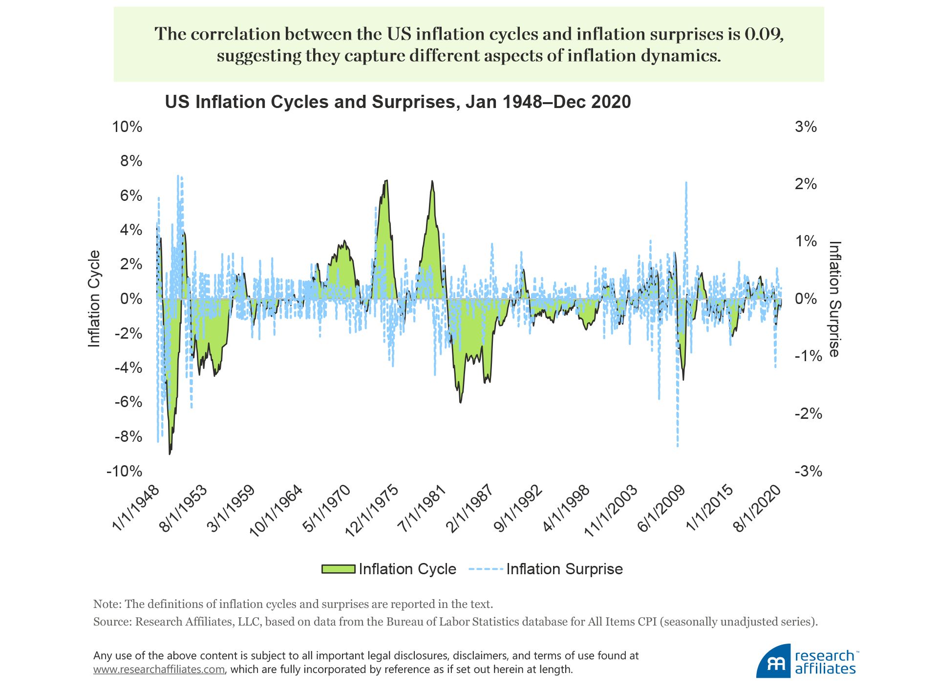
Cooper and Priestly (2009) document that positive output gaps associate with future lower equity excess returns. Consistent with their work, we expect that positive inflation signals should also associate with lower risk premia. In addition, because of the changing nature of inflation dynamics, we expect inflation surprises to display stronger predictive power in the earlier part of our sample, whereas inflation cycles should perform better over the last three decades.
Timing the US Equity Market with Inflation Signals
We convert inflation cycles and surprises to investment signals by constructing binary variables: +1 if the cycle or surprise is positive (rising inflation), and –1 if it’s negative (falling inflation). We call these \(s_{t}^{c}\) and \(s_{t}^{s}\) for cycles and surprises, respectively. Equipped with these two signals we simulate the returns of two self-financed portfolios that trade the US equity market. If a signal was negative (falling inflation), our strategy buys equities and finances the position with the one-month Treasury bill. If the signal was positive (rising inflation), the strategy sells the market and invests in the risk-free rate. The goal of the strategy is to profit by going long equities when inflation has been falling and by shorting them otherwise. The equity data start in January 1948 and are from the Kenneth French website, while the inflation data are from the Bureau of Labor Statistics. We employ seasonally unadjusted All Items CPI, which is an unrevised series, and in the portfolio tests we lag the inflation signals by two full calendar months to avoid look-ahead biases (we provide more details in Appendix B).
To test the strategy, we create portfolios based on the lagged inflation-cycle and inflation-surprise signals, which we label Cycles Portfolio and Surprises Portfolio, and also create a portfolio that is their average (Average Portfolio). As points of reference, we compare the returns of these portfolios with the excess returns of a long position in the equity market as well as a time-series momentum portfolio (TSMOM), which goes long, neutral, or short based on the sign of trailing 1- and 12-month excess returns.5 The alpha of the portfolios are calculated with respect to a simple long position in the equity market, and we report their statistical significance (t-Statistic). We summarize our evidence in the following table:
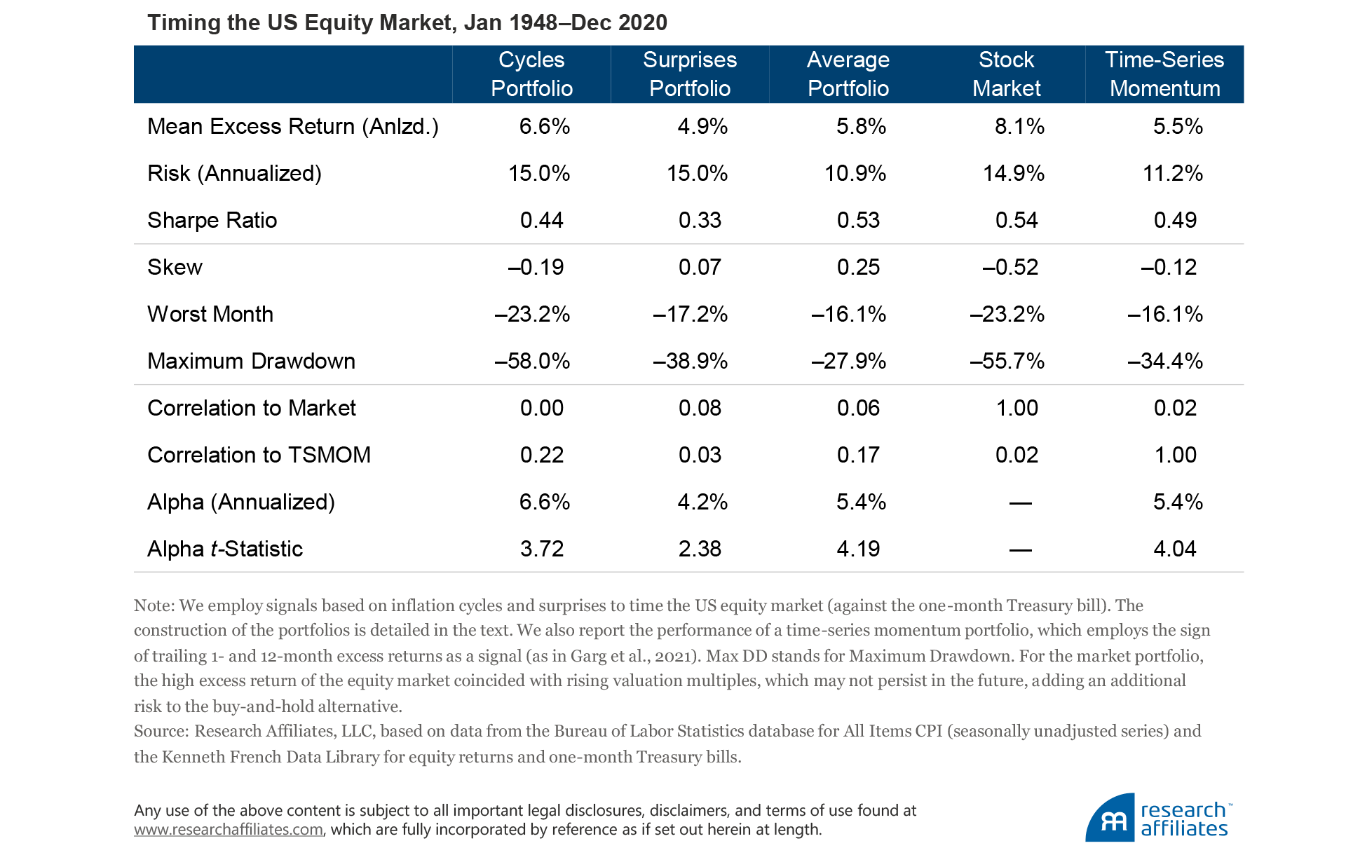
Our evidence suggests that inflation signals are indeed significant predictors of equities’ excess returns. Both signals translate into statistically and economically meaningful alpha; the cycles signal delivered the strongest outperformance. In particular, the premium harvested from combining the inflation signals is comparable to the one earned by the well-documented time-series momentum portfolio, while the two strategies themselves are mildly correlated (0.17).
Inflation signals are indeed significant predictors of equities’ excess returns. Both signals (cycles and surprises) translate into statistically and economically meaningful alpha.
”We highlight how the inflation signals capture different dynamics of the equity market. The correlation between the two tactical portfolios stands at only 0.02, so the Average Portfolio delivers higher risk-adjusted excess returns. In addition, the “lives” of the cycle and surprise signals are quite different. By construction, inflation cycles tend to persist over time, so the decay of the signal is relatively slow. In contrast, the decay of inflation surprises is much faster, because the signal displays little persistence, even over a monthly horizon.
Timing US Equity Sectors with Inflation Signals
Inspired by our market-level results, we move to a finer level of analysis by investing in individual equity sectors. Our prior is that different sectors should display different sensitivities (betas) to inflation signals and that these differences should translate into different performances across inflation regimes. Whereas all sectors may struggle following rising inflation rates, as Neville et al. (2021) document, some sectors may struggle more than others. The evidence shows exactly that.
We summarize the sensitivity to cycle and surprise metrics across 10 sectors as well as the aggregate market and across two periods (before and after 1990).6 For each sector j and the market, we run individual regressions of excess returns \(\textit{R}_{t+1}^{j}\) on the signals of cycles (\(s_{t}^{c}\)) or surprises (\(s_{t}^{s}\)). We then report the t-statistic associated with these relationships. As expected, both inflation signals are negatively associated with future excess returns across all sectors, meaning rising inflation corresponds to falling returns.
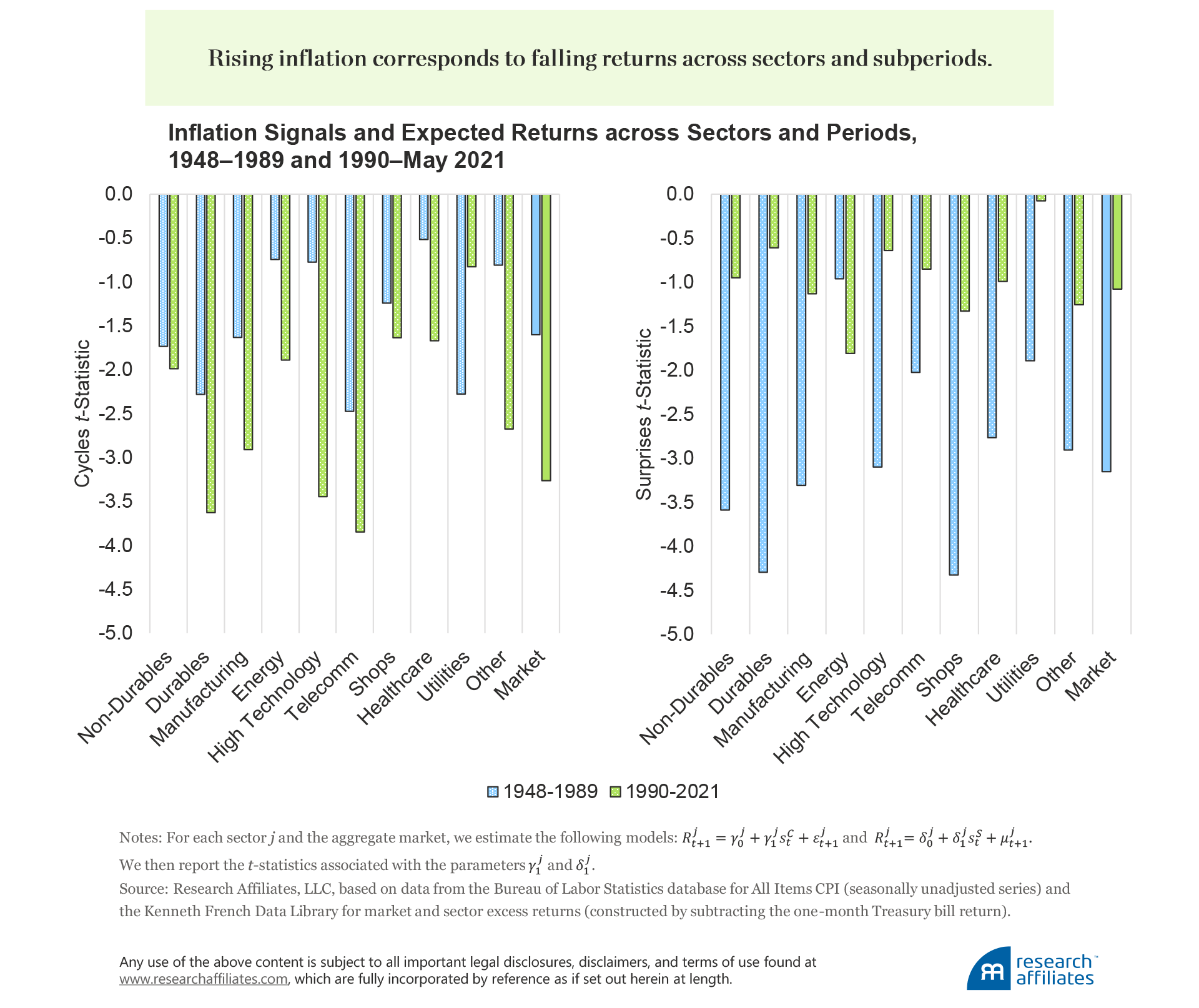
As hypothesized in the previous section, the sensitivity to cycles and surprises does indeed vary across decades. In recent years, inflation cycles have become a stronger predictor, whereas surprises have lost the lion’s share of their significance. These patterns are present across the majority of the sectors. We infer that, for the most recent decades, inflation expectations can be better approximated by employing moving averages with longer look-back windows; the opposite is true for the period of the 1970s and 1980s.
We also highlight some intuitive differences across sectors: the relationship with inflation signals tends to be the strongest for durables, which includes the automobile sector, and least successful for the energy-related sectors: energy and utilities. In general, these patterns can be explained via a complementarity channel. Inflation measures the changing price of different goods and services produced by different industries. Some of them are complementary goods, such as gasoline and cars, for which a price increase in one good leads to a decrease in the demand of the other good (an effect known as negative cross-elasticity of demand). We argue that the most predictable industries display the highest degree of complementarity to energy goods and services, and therefore struggle the most during periods of rising inflation. Yet, exceptions may occur, as in the case of tech firms, for which the duration channel is the most likely driver of sensitivity to inflation.
This dispersion of predictability across sectors motivates us to test a novel sector-rotation strategy. Our goal is to assess whether an investor could learn and exploit the dispersion in predictability in order to maximize the information contained by inflation-based signals. For both of our inflation signals, the design of our portfolio exercise is as follows:
Step 1. Every month using data from the previous 20 years, and for each sector, we estimate the predictive beta \(\beta^{j}\), where \(R_{t-1}^{j}=\alpha^{j}+\beta^{j} s_{t-2}+\mu_{t}^{j}\) and \(s_{t-2}\) is an inflation signal.
Step 2. We rank the betas for all sectors and generate 10 corresponding buckets: bucket #1 includes the sector with the highest (least negative) \(\beta^{j}\) each period, whereas bucket #10 includes the sector with the lowest (most negative) beta.
Step 3. For each bucket, we implement the following strategy: if \(s_{t-2}>0\), sell the bucket and invest the proceeds in the one-month Treasury bill; if \(s_{t-2}<0\), the strategy does the opposite.
In the following table, we report the average premia earned by cycle and surprise signals across buckets sorted by their trailing predictive beta. In the last column, we also report the L-H portfolio, which stands for low-beta minus high-beta portfolio. The portfolio is computed by taking the average of the five tactical portfolios with the most negative predictive betas—#6, #7, #8, #9, and #10—and subtracting the average of the five tactical portfolios with the least negative predictive betas (#1, #2, #3, #4, and #5). In brief, we do notice a monotonic relationship between the beta ranks and the performance of the timing strategies. The skewness and maximum drawdown statistics, which capture the tail properties of the strategies, also tend to improve with higher-ranked buckets. Hence, investors can successfully guess in advance for which sectors the timing strategy is expected to deliver the best returns.
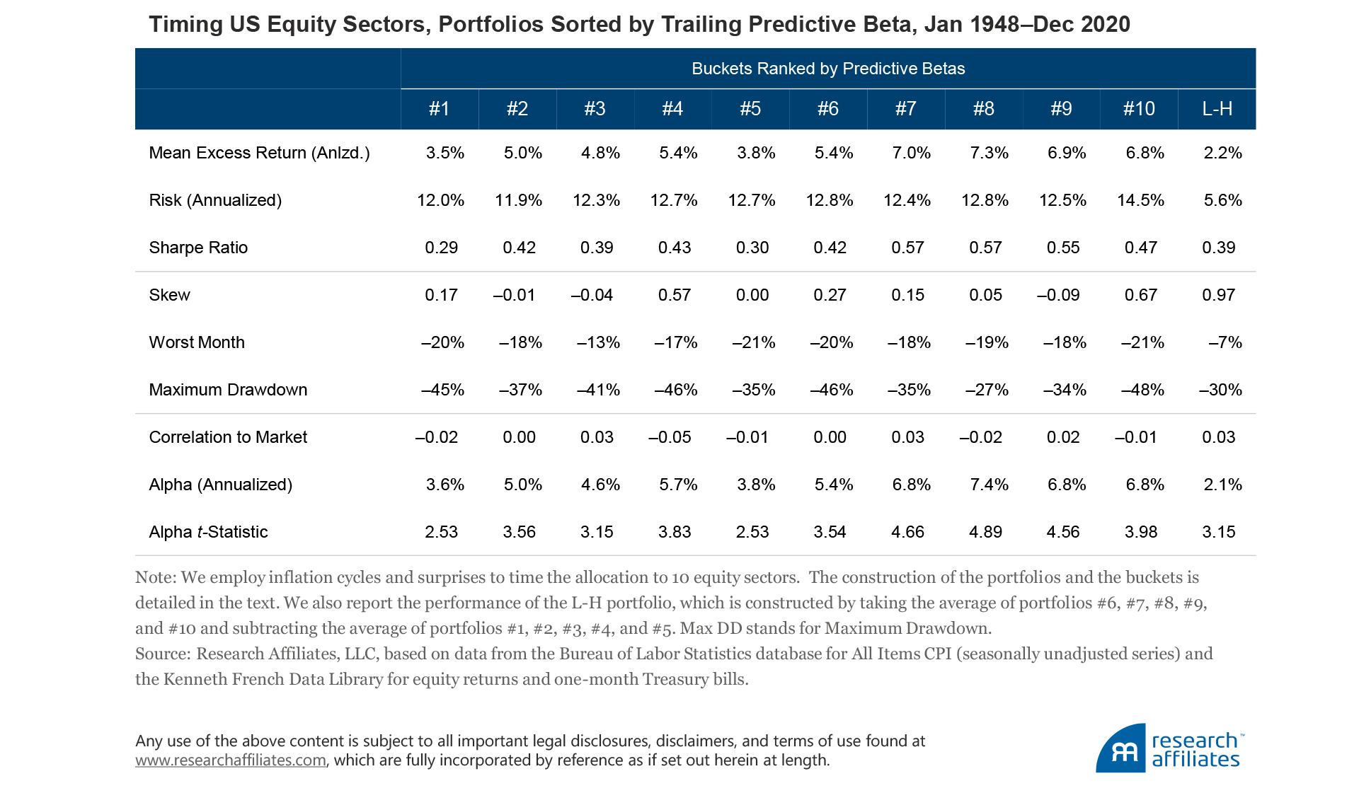
The L-H portfolio shows that these insights can be translated into a meaningful sector-rotation strategy. When inflation is trending downward, the L-H portfolio buys sectors with the lowest predictive betas and sells sectors with the highest betas, and it does the opposite when inflation is on the rise. This strategy is cross-sectional in nature—no use of the one-month Treasury bill—and delivers a statistically meaningful alpha with respect to the market.
Hedging Properties of Inflation Signals
In this last section, we document that inflation signals tend to provide protection against the worst economic times, regardless of whether they are driven by inflationary or deflationary pressures.
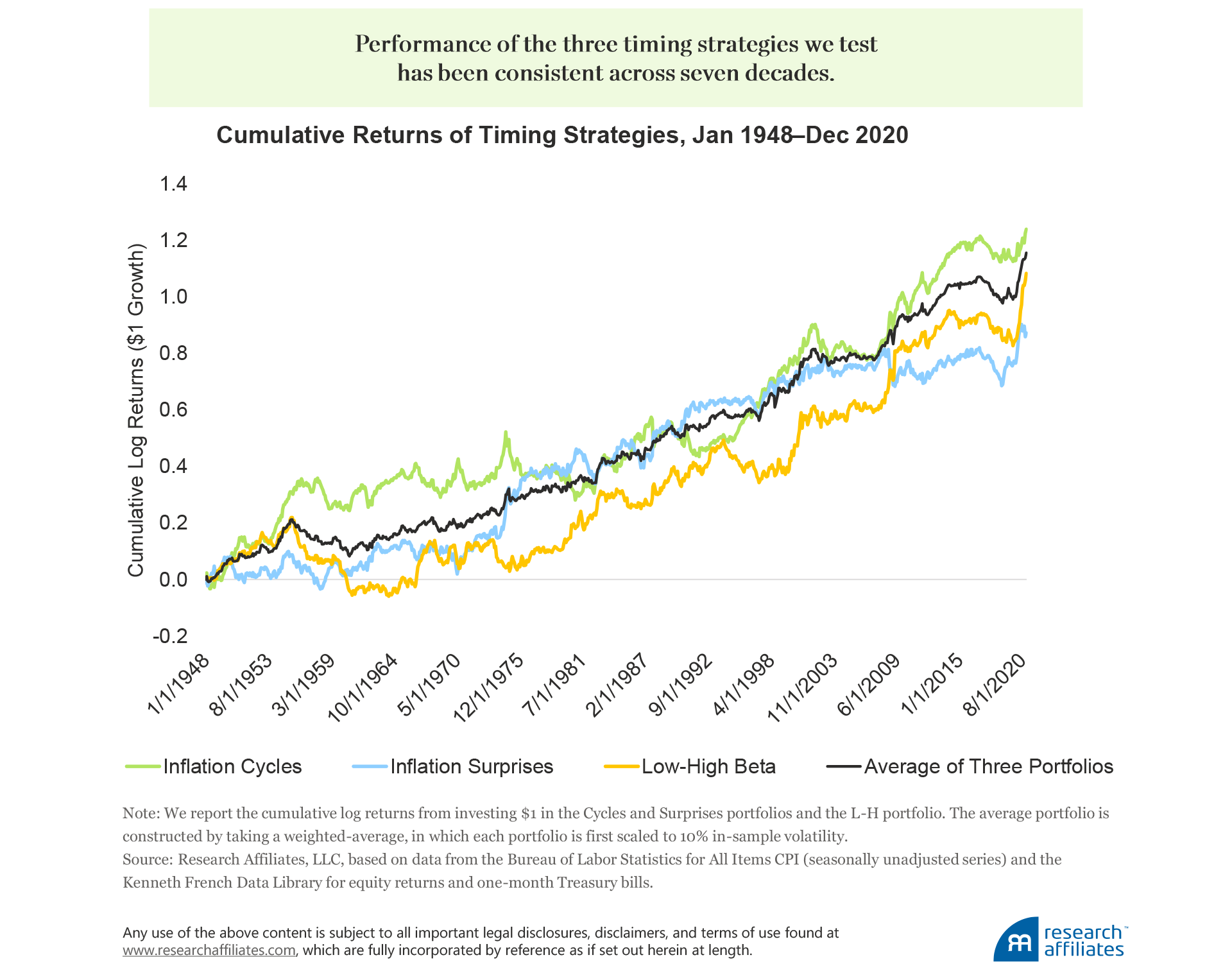
We plot the cumulative excess returns of three tactical portfolios—the Cycles and Surprises portfolios and the L-H portfolio we describe in our sector-rotation strategy—and their weighted average. In a nutshell, their performance has been consistent across seven decades. The correlations of the three portfolios are below 0.20, indicating that the diversified average portfolio delivers a particularly solid performance (Sharpe ratio of 0.59 and an alpha t-statistic of 4.63).
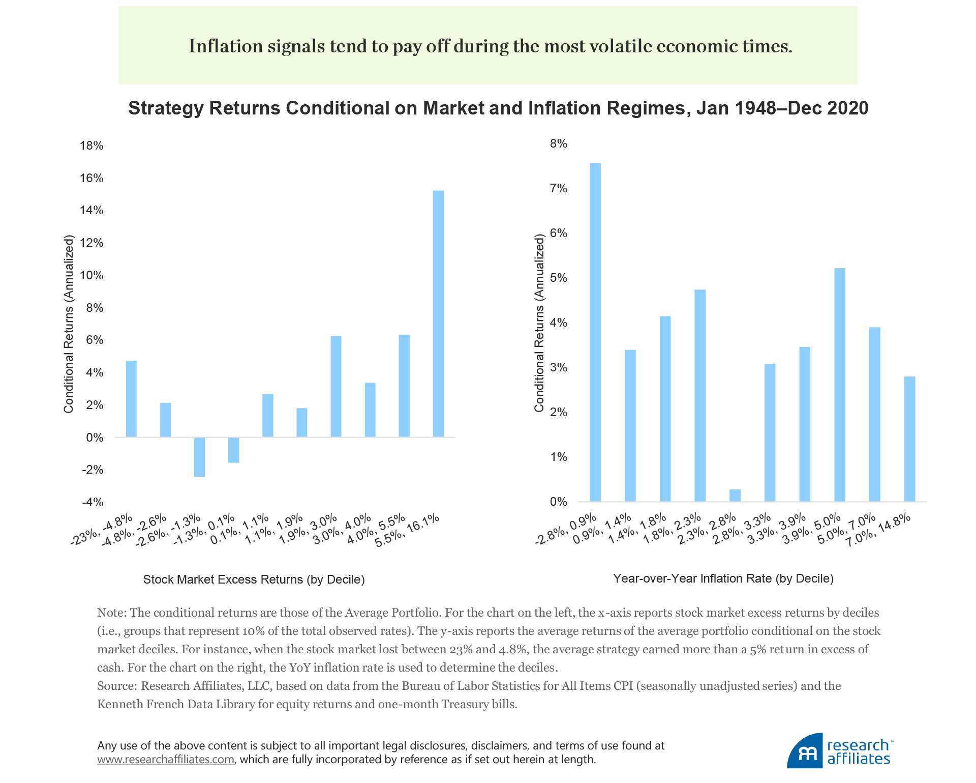
Next, we calculate the excess returns of the average of the three portfolios, conditional on the stock market’s contemporaneous performance and the year-over-year inflation rate. The signals provide remarkable protection against market tail events—short when the market tanks, and long when it rallies—as well as offering consistent performance across inflation regimes.7 Similar to trend-following strategies, portfolios based on inflation signals display a payoff profile akin to that of an option straddle on the market. More generally, inflation signals tend to pay off during the most volatile economic times.
We interpret the hedging properties of inflation signals by leveraging their underlying economic motivation—the Phillips Curve. Our research shows that positive values of the average of the cycle and surprise signals tends to predict economic contractions over the subsequent year, whereas negative values tend to predict economic expansions. Hence, the average signal should deliver long positions when a new bull market is established, whereas it should recommend short positions during bear markets.
Conclusion
In this article, we document that two derived US inflation variables—inflation cycles and inflation surprises—have been robust predictors of US equity returns. We demonstrate that this predictability translates into new sources of alpha that investors can seek to harvest. In particular, we highlight the signals’ ability to perform during the worst times in the stock market without missing upside opportunities.
The tail-hedging properties derived from inflation signals are particularly desirable. Hedging positive inflation shocks can be costly when inflation is low.8 For example, strategic allocations to alternative assets, such as commodities, or absolute return strategies as a way to protect against inflation have not all fared well in recent years, with commodity indices down more than 30% versus their 2011 levels. As a result, many asset owners may not be able to stay the course if inflation fails to materialize in the medium term. We find that inflation signals can provide a new tool for investors who wish to hedge their portfolios against inflationary and deflationary risks.
Appendix A: Extracting Signals from the Phillips Curve
The Phillips Curve is a reduced-form equation that connects the current inflation rate to inflation expectations and the business cycle. To empirically fit the Phillips Curve, economists found success by assuming that inflation expectations are approximated by a weighted-average of past inflation rates (the so-called accelerationist version of the curve). This approach follows the steps of the constant-gain learning literature and is consistent with the modeling approaches of the inflation- and bond-forecasting literature (e.g., Faust and Wright, 2013, and Cieslak and Povala, 2015).
Hence, let \(\pi_{t}^{i}\) denote the year-over-year inflation rate of index i measured on month t; define yt as a generic term representing the state of the economy (such as the output or unemployment gap); and define a weighted-average of past inflation rates, \(\bar{\pi}_{t}\), as \[\bar{\pi}_{t}=(1-v)\sum_{n=0}^{t-1}v^{n}\pi_{t-n}\]
We can rewrite the Phillips Curve as follows: \[\pi_{t} - \bar{\pi}_{t-1}=\delta+\rho\textit{y}_{t}\]
where δ and ρ are parameters that further model the relationship. Our insight is that the difference, \(\pi-\bar{\pi}_{t-1}\), can be interpreted as a proxy for the state of the economy (yt in our equation) and can be employed as a predictor of equities’ excess returns.
To translate an economic concept into an actionable investment strategy, we need to choose the starting month of the sample as well as the parameter v of the weighted-moving average, \(\bar{\pi}_{t}\). We solve the question of the starting sample by simply truncating the sum at 120 months, so we effectively compute a weighted average of past inflation rates over a 10-year rolling window.
Pertaining to the calibration of the v parameter, we consider two solutions that span the spectrum of options between 0 and 1. First, we set \(\bar{\pi}_{t-1}=\pi_{t-1}\), from which it trivially follows that \(\pi_{t}-\bar{\pi}_{t-1}=\pi_{t}-\pi_{t-1}\). In this case, the inflation differential amounts to what we call an inflation surprise, the monthly change in year-over-year inflation rates. This signal is almost indistinguishable from a calibration of v that approaches zero. Second, we set v = 0.99, for which the term \(\bar{\pi}_{t}\) resembles a smoother 10-year moving average. Given its slow-moving nature, we label this definition of \(\pi_{t}-\bar{\pi}_{t-1}\) an inflation cycle. When setting v = 0.99, we ensure that the sum of the weights of the moving average adds up to 1.
Appendix B: Details on Inflation Data
With respect to the other macro variables, the headline inflation index (CPI-U) has the key advantage of not being subject to revisions. As Croushore and Stark (1999) explain, the CPI is “revised only through changes in seasonal adjustment factors or changes in the base year.” As they point out, the seasonally unadjusted CPI series can be employed for forecasting purposes without concern regarding revisions.
Throughout our research, we utilize only seasonally unadjusted CPI data obtained from the Bureau of Labor Statistics website. The series for headline inflation starts in January 1913. Over the last 20 years, inflation has been typically released during or at the end of the second week of a month. Earlier in the sample, inflation data were released with a slightly greater delay of about three or four weeks. For instance, the year 1953 is the first year for which we have a historical record available.9 During that year, inflation statistics were released between the 22nd and 27th of the subsequent month. Hence, lagging inflation signals by two full calendar months should alleviate concerns of look-ahead biases.
Please read our disclosures concurrent with this publication: https://www.researchaffiliates.com/legal/disclosures#investment-adviser-disclosure-and-disclaimers.
Endnotes
- The literature that has documented this empirical regularity includes Fama and Schwert (1977), Fama (1981), Lin (2009), Bekaert and Wang (2010), Bekaert and Engstrom (2010), and Neville et al. (2021). The selected index in these studies is the All Items Consumer Price Index (CPI), which offers the longest series of data (in contrast to breakeven inflation rates, whose history is relatively short). In this article, we follow the literature and exclusively focus on All Items CPI (seasonally unadjusted series).
- To compute cycles and surprises, we could employ surveys to approximate investors’ inflation expectations. On the one hand, surveys have the benefit of being forward looking in nature and unrelated to a particular model. On the other hand, they tend to display a relatively short history and may be released at lower frequencies. In general, our research finds that computing cycles and surprises with moving averages or surveys leads to very similar signals. Hence, given the longer history and higher frequency of metrics based on trailing data, we opt for computing cycles and surprises by employing moving averages. Market-based expectation signals, such as breakeven inflation and inflation swaps, also suffer from short histories as well as embedded risk premia.
- For instance, the autocorrelation of the quarter-over-quarter rate of inflation was 0.63 over the period January 1948–December 1989. It fell to −0.11 over the period January 1990–May 2021 (computed using quarterly frequency data).
- Related to this point, we note that the evidence we present that the equity market has underperformed when inflation was relatively high is not obviously translatable to an investment strategy. Indeed, the mean of the inflation rate has varied across decades as has the notion of “high” and “low” inflation. A sustained rate of 5% inflation is arguably high in today’s world, but was not out of the ordinary just 30 years ago. Inflation cycles and surprises are related to the direction of the inflation rate, rather than to its level.
- Time-series momentum (or trend-following) is a well-documented phenomenon across financial markets and is at the core of the CTA/Managed Futures industry (e.g., Moskowitz et al., 2012). In its simplest form, the strategy goes long an asset and short cash if the trailing excess returns of the asset are positive, and it does the opposite otherwise. In this article, we employ trailing 12-month excess returns to determine portfolio positions, which constitutes a common benchmark in the literature.
- The choice of 10 sectors is motivated by the desire to approximate the financial industry’s own definition of sectors (see, for instance, the Global Industry Classification System by MSCI). We note, however, that our results are robust to choosing a larger universe of sectors.
- The Average Portfolio’s positions are inversely related to inflation (positive when inflation is relatively low, and negative otherwise). Thus, the positive excess returns earned by the Average Portfolio when inflation is in the top four deciles (above 3.3%) are obtained by being, on average, net short the equity market.
- Similar to an insurance premium, the investor pays a premium in “normal” times to protect their portfolio against an adverse event.
- Historical release data are available at https://www.bls.gov/bls/histreleasedates.pdf.
References
Bekaert, Geert, and Eric Engstrom. 2010. “Inflation and the Stock Market: Understanding the ‘Fed Model’.” Journal of Monetary Economics, vol. 57, no. 3 (April):278–294.
Bekaert, Geert, and Xiaozheng Wang. 2010. “Inflation Risk and the Inflation Risk Premium.” Economic Policy, vol. 25, no 64 (October):755–806.
Cieslak, Anna, and Pavol Povala. 2015. “Expected Returns in Treasury Bonds.” Review of Financial Studies, vol. 28, no. 10 (October):2859–2901.
Cooper, Ilan, and Richard Priestley. 2009. “Time-Varying Risk Premiums and the Output Gap.” Review of Financial Studies, vol. 22, no. 7 (July):2801–2833.
Croushore, Dean, and Tom Stark. 1999. “A Real-Time Data Set for Macroeconomists.” Working paper 99-4, Federal Reserve Bank of Philadelphia (June).
Fama, Eugene. 1981. “Stock Returns, Real Activity, Inflation, and Money.” American Economic Review, vol. 71, no. 4 (September):545–565.
Fama, Eugene, and G. William Schwert. 1977. “Asset Returns and Inflation.” Journal of Financial Economics, vol. 5, no. 2 (November):115–146.
Faust, Jon, and Jonathan Wright. 2013. “Forecasting Inflation.” In Handbook of Economic Forecasting, edited by Graham Elliott and Allan Timmermann, vol. 2A, 2–56. ScienceDirect.
Garg, Ashish, Christian Goulding, Campbell Harvey, and Michele Mazzoleni. 2021. “Momentum Turning Points.” Working paper (January 23). Available on SSRN.
Lin, Shu-Chin. 2009. “Inflation and Real Stock Returns Revisited.” Economic Inquiry, vol. 47, no. 4 (October):783–795.
Moskowitz, Tobias, Yao Hua Ooi, and Lasse Pedersen. 2012. “Time Series Momentum.” Journal of Financial Economics, vol. 104, no. 2 (May):228–250.
Neville Henry, Teun Draaisma, Ben Funnell, Campbell Harvey, and Otto Van Hemert. 2021. “The Best Strategies for Inflationary Times.” Working paper (May 25). Available on SSRN.
Williams, John. 2019. “Discussion of 'Prospects for Inflation in a High Pressure Economy: Is the Phillips Curve Dead or Is It Just Hibernating?'" by Peter Hooper, Frederic S. Mishkin, and Amir Sufi.” Remarks at the US Monetary Policy Forum, New York City (February 22).

