
The massive growth in central bank balance sheets via quantitative easing, debt monetization, and firing of “big bazooka” stimulus packages gives the business cycle a renewed level of importance for understanding how changes in growth and inflation impact future shifts in global asset markets.
We demonstrate the varying sensitivities of 15 asset classes to changes in growth and inflation. We show that a strategy employing these two metrics and currently available market data (i.e., no forecasting) can outperform a simple equally weighted portfolio.
Based on the leading indicators of our simple TAA strategy, we are in a period of below-trend growth and inflation, which implies that an overweight to nominal bonds and reduction in commodities exposure would be appropriate. Markets, however, have been supportive of the “reflation” trade. Our model indicates it may be too early to adopt the reflation trade, and some reversal may occur.
The business cycle is one of the most important concepts an investor should consider when constructing a portfolio of assets. Although we all have an intuitive awareness of the business cycle, economists and strategists use a wide variety of indicators to describe where the economy is in the cycle at any given time. For the purpose of this article, we extrapolate the business cycle in two dimensions: growth and inflation,1 and more specifically by increasing or decreasing rates of each metric.
The business cycle has always been an important force in investment decision making, but the massive growth in central bank balance sheets via quantitative easing, debt monetization, and firing of “big bazooka” stimulus packages may give the business cycle a renewed level of importance in the years ahead. Revisiting this topic now provides a basis for thinking about potential future shifts in global asset markets.
We show in a multi-asset context that different asset classes have varying sensitivities to changes in growth and inflation. We also show that a strategy that employs these two metrics and currently available market data (i.e., no forecasting) can outperform a simple equally weighted portfolio. We find that a great deal of information about future asset returns is available just by knowing the current stage of the business cycle. Our results help illustrate why growth and inflation are informative to asset returns and open the door to more-advanced forecasting techniques that can capture the additional theoretical benefits in knowing which business-cycle stage is up next.2
After presenting evidence on how our macroeconomic-regime approach performs, we will review the stage of the business cycle we are in today and what it implies for portfolio positioning. We recommend an overall awareness of the effect of potential macroeconomic “shocks” in the road ahead as an important input to guide investors’ tactical asset-allocation decisions toward better long-term outcomes.
Growth and Inflation Sensitivities
Before delving into the macroeconomic regimes formed by the intersections of increasing and decreasing rates of growth and inflation, we consider each of the variables (growth and inflation) independently using a set of market indices to model the dynamics of 15 asset classes.
We calculate the return of each asset class in excess of its average return over the period January 1960–December 2020 in the months when real GDP growth was above and below trend growth (i.e., when real GDP is accelerating or decelerating relative to a rolling five-year trend). We describe the months in which this relationship occurs as a GDP shock.
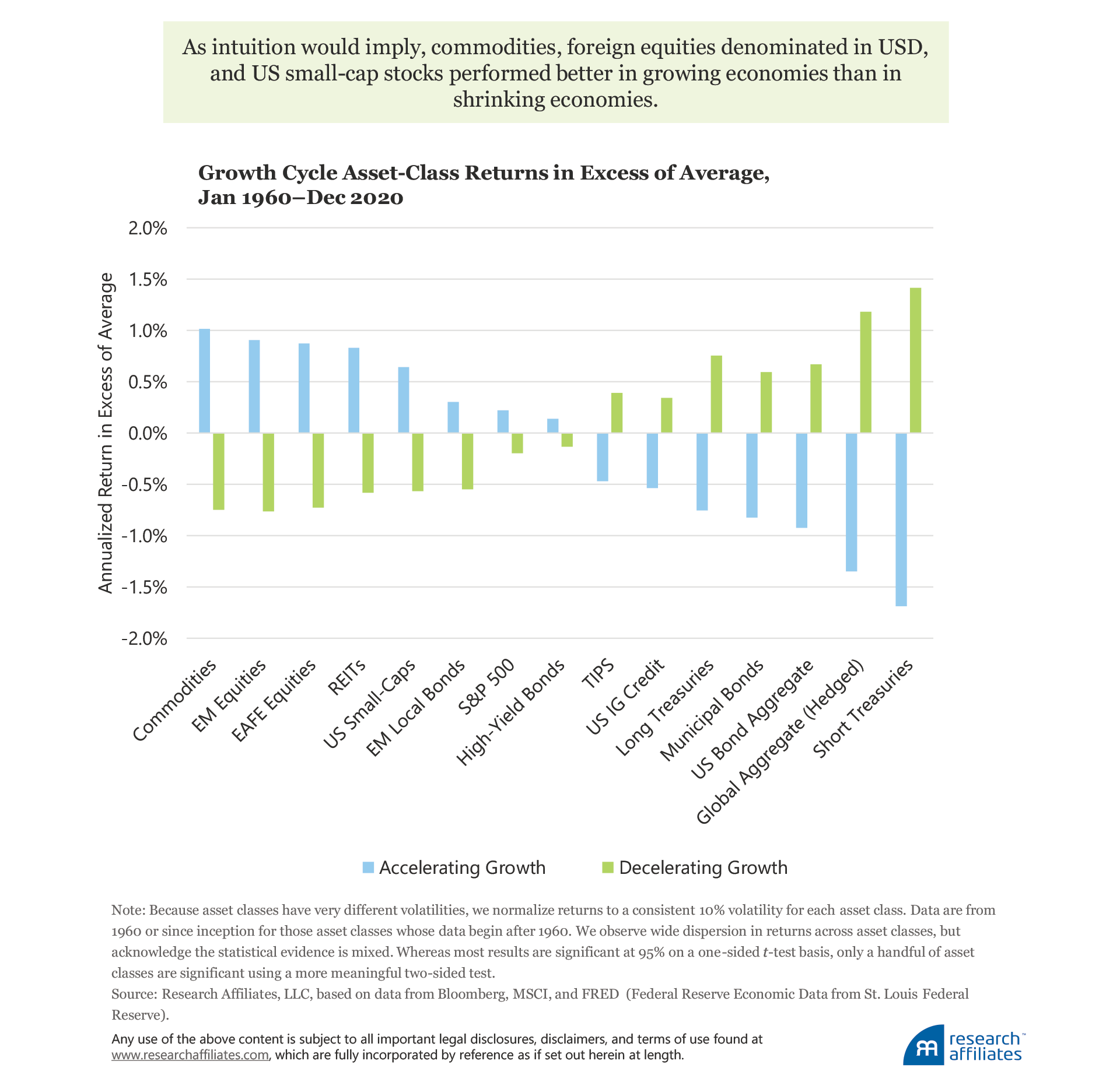
Adding credence to our measurement of growth are intuitive results across many of the asset classes in our sample. For example, US small-cap stocks, foreign equities denominated in USD, and commodities had a higher average return in times of higher-than-average growth than they did in times of negative shocks. Conversely, bonds, most notably short-term government bonds, outperformed in months when growth was contracting. No surprise then that the performance of asset classes having both stock and bond qualities, such as investment-grade and high-yield bonds, fell somewhere in the middle, producing less-significant results.
Interestingly, the variations in S&P 500 Index returns when controlled for growth-shock periods are not as consequential under our definition as we would have thought a priori, although the results are in the direction we would expect. We did consider using the leading indicator metric from the OECD (Organisation for Economic Co-operation and Development), but because that metric is typically delayed for months and then often revised, we prefer our definition. Our definition captures the proper direction of the next macroeconomic regime with the added benefit of reducing data delay.
Now, let’s turn our attention to inflation by performing a similar analysis, but first we need to define what we mean by inflation. For those who remember the US inflationary environment of the 1970s and early 1980s as well as periods of hyperinflation experienced by other nations, the term inflation brings back memories of double-digit inflation, unseen in the United States since that time. Therefore, a focus on periods of high inflation would not be very useful for today’s investors.3 Instead, as with growth, we examine periods of rising and falling inflation from January 1960 through December 2020 defined as those months when rates of change are above or below trend inflation. We describe such an interval as an inflation shock.
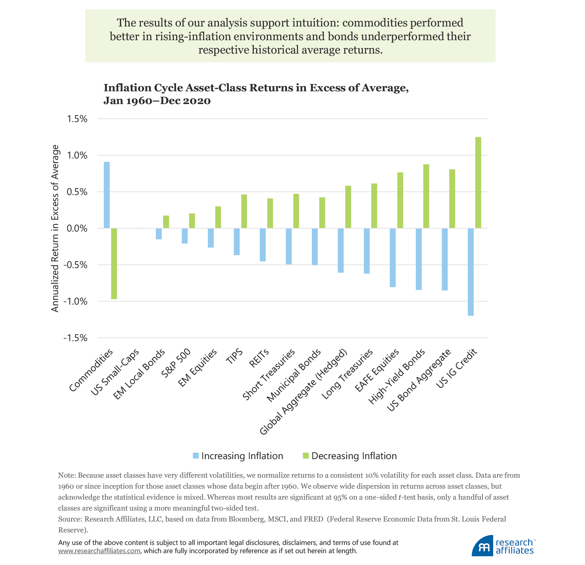
As with growth, certain results consistent with intuition add to the credence of our measurement technique. For example, commodities performed better in rising-inflation environments. On the flip side, fixed-rate investments, Treasury and investment-grade bonds, and foreign stocks all underperformed their respective average return in positive inflation-shock environments. We find that inflation protection from TIPS (Treasury Inflation-Protected Securities) has been suspect, consistent with the findings of Ang (2012).
Combining Growth and Inflation
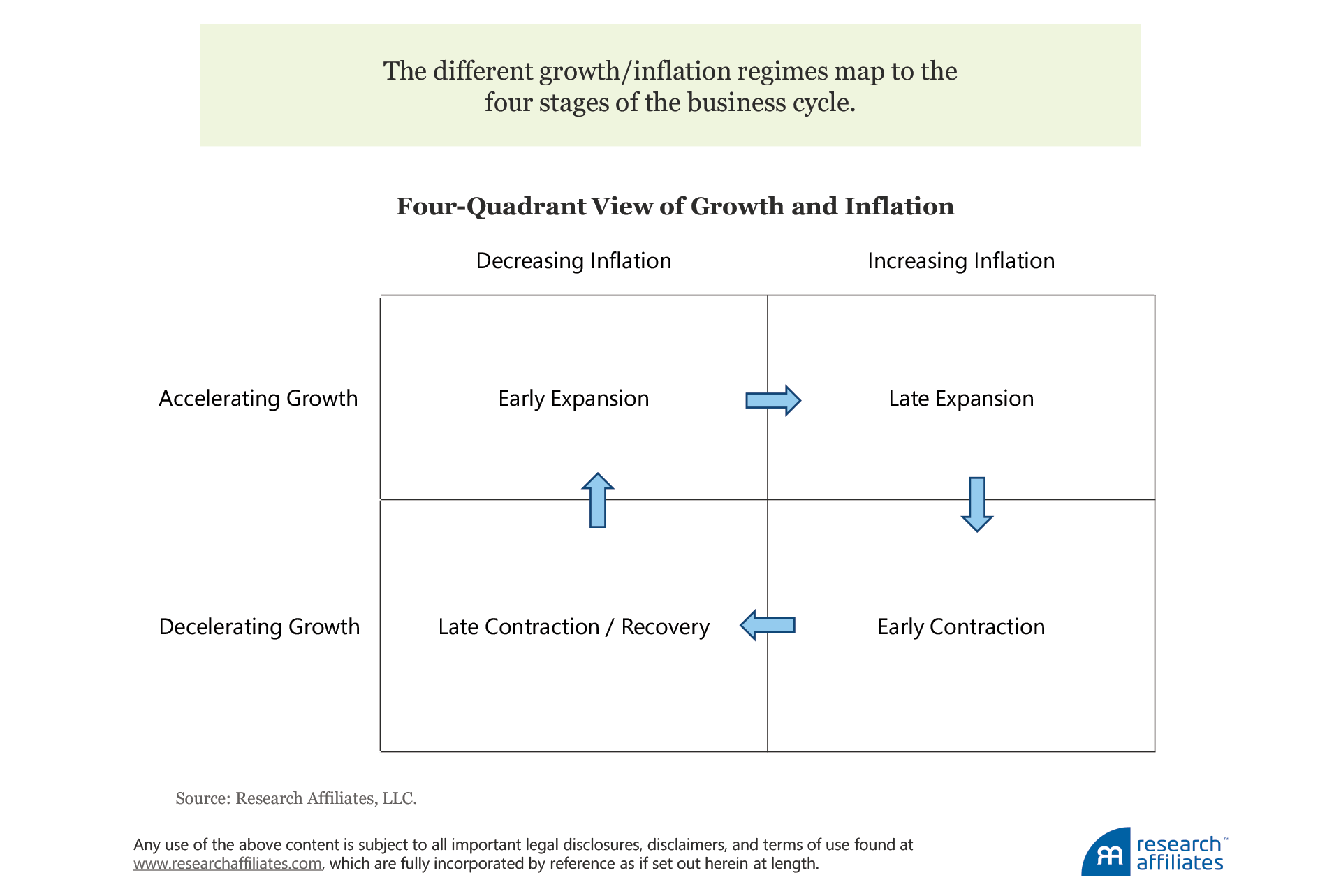
Thus far, we have assessed how each of the 15 asset classes performed in periods of accelerating and decelerating growth and inflation relative to their five-year trend over the 1960–2020 period. Now, we combine these two variables to describe the four stages of the business cycle. Each of the stages maps to a combination of accelerating or decelerating inflation or growth, typical of what the economy normally experiences during these stages. For example, following an economic downturn, the next stage is expansion, which usually begins with accelerating growth and stable or falling inflation. In the next stage (late expansion), inflation increases as the expansion continues, before growth turns negative during the early part of a contraction. In late contraction/recovery, both variables decrease before the cycle starts anew.
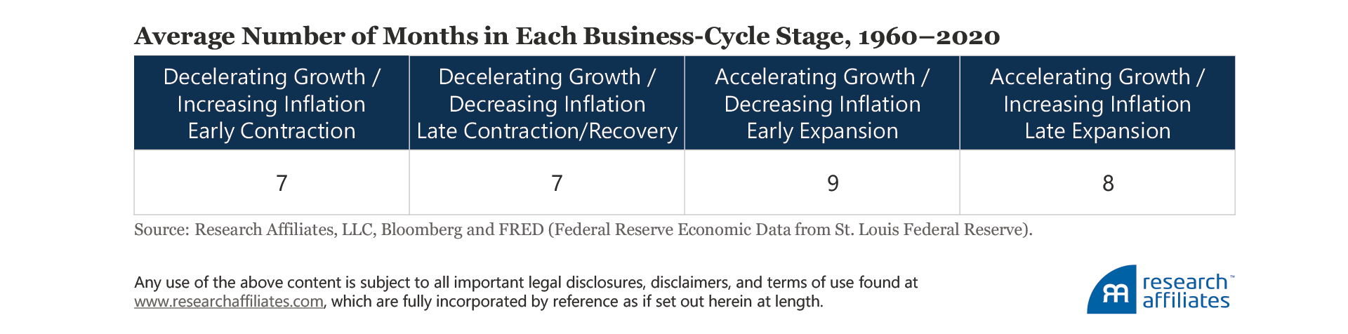
Ideally, in mapping these two variables to the stages of the business cycle, we would gain confidence by observing persistence. After all, the business cycle does not normally jump between stages month over month, whereas simple measures of growth and inflation might do just that. We do in fact observe persistence, given that the average number of months in each stage is about eight (or three quarters), meaning a full four-stage cycle would last three years.
To determine how an investor could profit from the business-cycle framework we set forth, we employ a strategy that tactically allocates among four asset classes, using an index as a proxy for each: US equities (S&P 500 Index), US investment-grade bonds (Bloomberg Barclays Aggregate Bond Index), commodities (S&P GSCI Index), and TIPS (Bloomberg Barclays US TIPS Index). We selected these four asset classes because economic theory suggests that, given their return drivers, they should perform well and/or poorly during the various growth/inflation states.
Our choice of the S&P 500 and TIPS indices might seem odd because these asset classes did not have notable positive/negative returns compared to their respective historical return averages in our earlier analyses of asset class returns over growth cycles and inflation cycles. Nevertheless, we selected them (instead of developed-market equities or US small caps, for example, which did show notable returns versus their historical average returns) because many investors, who do not have the benefit of our analysis, hold these assets based on expectations of positive returns over changing growth and inflation regimes. We are attempting to model real-world investor holdings.
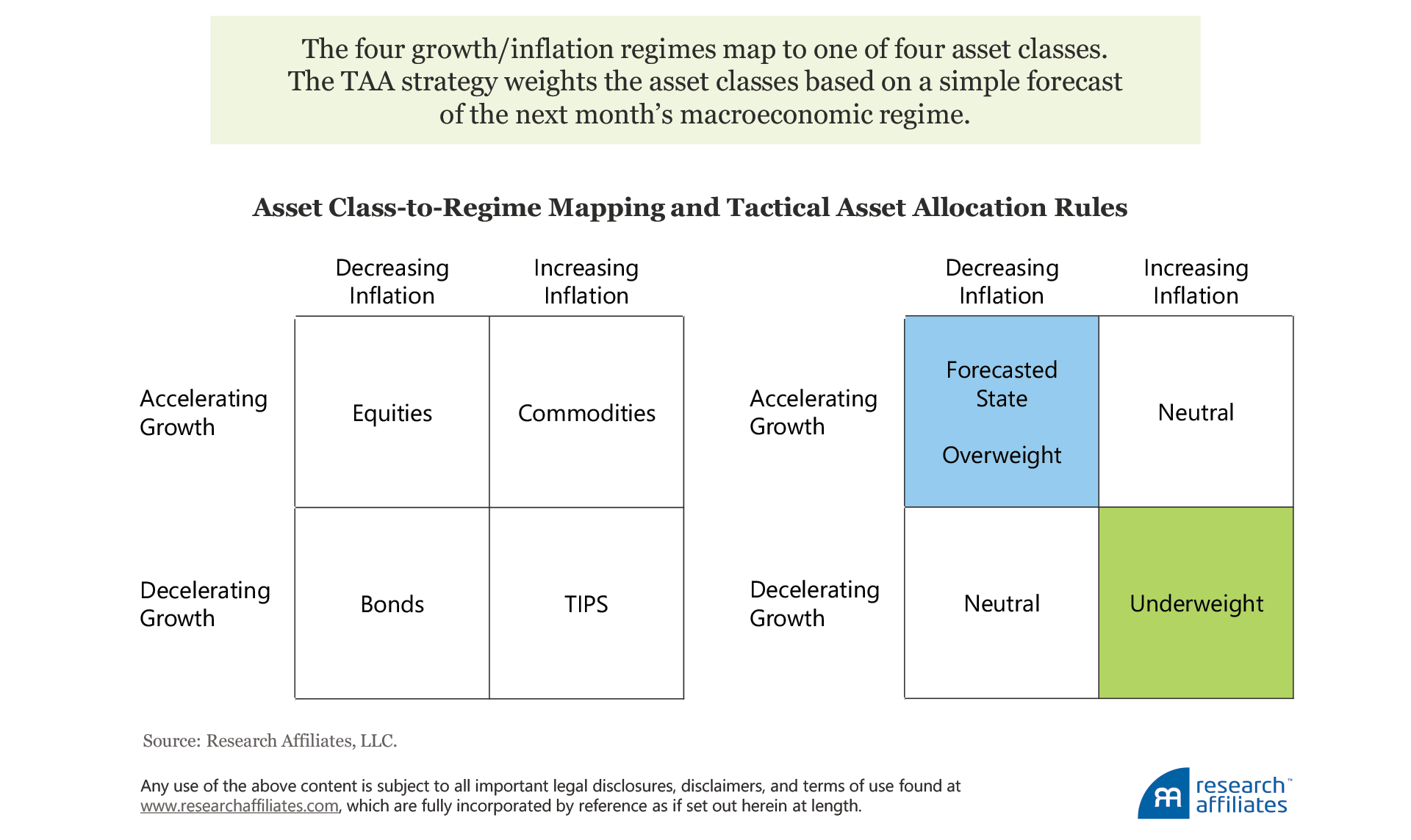
We construct an equally weighted benchmark that allocates 25% to each of the four asset classes. We also construct a tactical asset allocation (TAA) strategy by mapping each asset class to one of the four quadrants as follows: accelerating growth/decreasing inflation (equities), accelerating growth/increasing inflation (commodities), decelerating growth/increasing inflation (TIPS), and decelerating growth/decreasing inflation (bonds). We increase the weight of the asset class if our expectation of growth and inflation in the next business-cycle stage aligns with that asset’s quadrant. The asset class mapped to the quadrant that is diagonal from the overweighted quadrant is underweighted.
The over/underweight amounts are 25%; in other words, we allocate 50% to the overweighted asset class and 0% to the underweighted asset class. The asset classes mapped to the two off-diagonal quadrants remain neutral at a 25% allocation to each. For example, if the next month’s macroeconomic forecast is for accelerating growth and decreasing inflation, the allocation to equities increases from 25% to 50%, the allocation to TIPS decreases from 25% to 0%, and the allocation to bonds and commodities remains at 25% each.
Because the purpose of our analysis is to focus on growth/inflation regimes and not on complex trading algorithms, we chose the simplest trading rules we could devise.
The backtest for the TAA strategy spans January 1997 through December 2020. In the appendix, we provide results from a backtest that begins in 1976, and which required the modeling of synthetic assets such as TIPS. In each backtest, we rebalance monthly both the equally weighted benchmark and the tactical strategy portfolio. The macroeconomic regime expectations we described previously drive the tactical strategy.
Growth and Inflation “Forecasts”
Our tactical asset allocation strategy is simple at first glance but lacks a key component, namely, a method to identify the expected growth/inflation regime for the next month. Many models and methods for forecasting growth and inflation exist, but in order to reinforce the value of our macroeconomic framework, we take a very simple approach. Our forecast for the next growth/inflation regime follows a random-walk model. This serves two purposes: first, it simplifies our analysis so we can focus on the tactical allocations, and second, it serves as a benchmark for future extensions of this research that might utilize more-complex models.
We constructed monthly macroeconomic regime forecasts. With an awareness that macroeconomic data are often revised and are typically published with a delay, we appropriately adopted a lag in regime observations, and consequently, our forecasts. We lag the growth-regime variable by six months and the inflation-regime variable by one month (we found no meaningful difference when the lag was two months). Our forecast for the next month’s macroeconomic regime thus becomes the combination of these two lagged variables. We also constructed a hypothetical portfolio based on a set of “perfect” forecasts (i.e., perfect foresight) in order to disentangle the value-add of the TAA strategy from the simple forecasts.
TAA Strategy Results, January 1997–December 2020
When evaluating the performance of our backtest TAA strategy, we examined a wide range of portfolio characteristics including risk–return reward, drawdown, and distribution of returns and weights. Over the January 1997–December 2020 period, the tactical strategy’s risk-adjusted return profile (Sharpe ratio of 0.56) is favorable compared to that of the equally weighted benchmark (Sharpe ratio of 0.37). In addition, the tactical strategy’s maximum drawdown is lower than the maximum drawdown of the equally weighted benchmark (−27% vs −34%, respectively), indicating the tactical allocations informed by macroeconomic regime forecasts have helped reduce painful drawdowns for investors; in this case, both maximum drawdowns occurred during the global financial crisis.
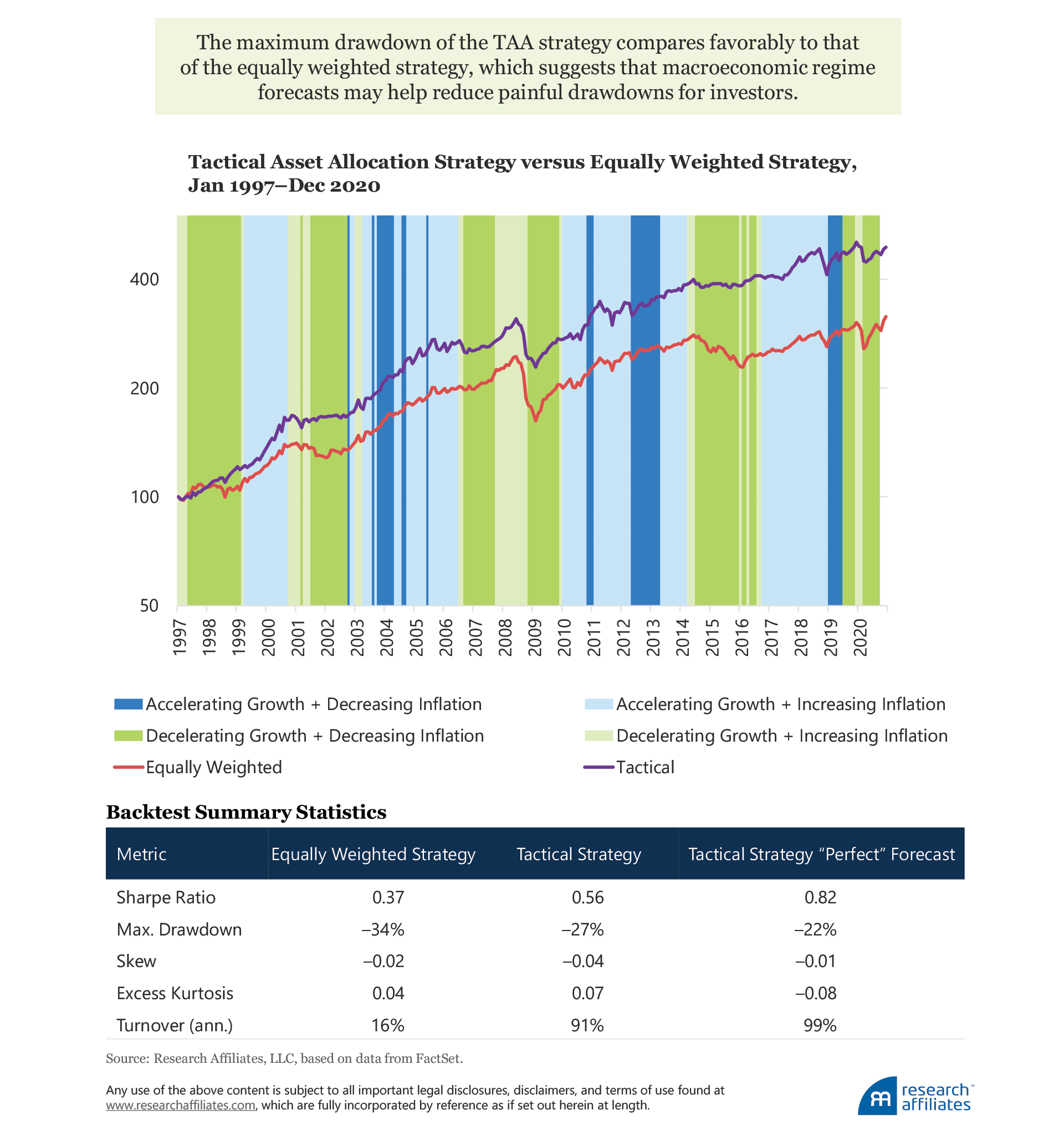
The favorable comparisons were achieved without significant deviations in the return distribution characteristics of the tactical and equally weighted strategies, including skewness (−0.04 versus −0.02, respectively) and excess kurtosis (0.07 versus 0.04, respectively). Unsurprisingly, turnover is much higher in the tactical strategy (91%) than in the simple equally weighted benchmark (16%), yet is still within reason for many investors. For the purpose of our simple horse-race proof of concept, we do not attempt any additional complexity with respect to turnover management.
For comparison purposes, we also look at the perfect-forecast TAA strategy, which has the benefit of exactly predicting the next business-cycle stage, and therefore captures the best-case conditions for the tactical strategy. Unsurprisingly, the perfect-forecast strategy provided even better performance metrics (e.g., higher Sharpe ratio and lower drawdown) compared to the TAA strategy, which simply utilizes the previous macroeconomic observation as a forecast for weighting the asset classes. Our simple growth/inflation forecasts correctly predict the next month’s macroeconomic regime approximately 67% of the time over the 1997–2020 backtest period. Therefore, our extremely simple random-walk method of “forecasting” growth and inflation leaves some meat on the bone, indicating additional value is available for extraction. The investor would need to decide if improving the forecast model through added complexity in order to harvest all or some portion of the remaining 33% of return was warranted.
Even with tactical allocations across the four asset classes, the TAA strategy does not have a significant tilt toward any particular asset class; the average asset allocations in the tactical strategy are 24% each to equities and bonds and 26% each to commodities and TIPS. In fact, an overall equity beta of 0.33 for the tactical strategy versus 0.37 for the benchmark suggests the tactical strategy does not outperform simply based on a structural loading on equity beta. On average, the strategy invests in each asset class as often as the equally weighted benchmark does (+/−1%).
Portfolio Results Deep Dive
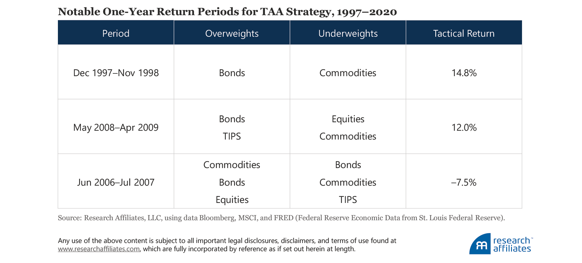
We take a closer look now to see in which macroeconomic environments the tactical strategy outperformed and underperformed the benchmark from 1997 through December 2020, and why. We examine three one-year periods when the TAA strategy had notable over- or underperformance versus the equally weighted benchmark. Given the tactical nature of the strategy, we observe instances when a given asset class is both under- and overweighted within the same one-year period.
December 1997–November 1998: During the Asian financial crisis that began at the end of 1997 and lasted nearly all of calendar year 1998, commodities suffered and the price of WTI crude oil declined from $30 a barrel at year-end 1997 to below $20 a barrel by November 1998. Our simple macroeconomic regime model correctly forecasted the decelerating growth/decreasing inflation regime for this entire one-year period. The long US bonds and short commodities tactical allocation provided an impressive tactical return of 15.0% over this one-year span.
May 2008–April 2009: For most of the global financial crisis when growth was decelerating, the TAA strategy underweighted equities. Of course, this underweight greatly benefited from the equity market crash, providing approximately 10.0% of the tactical return to the portfolio and leading to an overall tactical return of 12.0% over the one-year period from May 2008 to April 2009.
June 2006–July 2007: In this one-year period in the mid-2000s, the price of WTI crude oil pulled back from the mid-$90s a barrel to under $80 a barrel. Over this time, the TAA portfolio was overweight commodities, resulting in a −5.5% tactical return. The subsequent rebound in oil prices to an all-time high unfortunately coincided with the strategy's late underweight to commodities resulting in an additional −2.0% tactical return. The significant underperformance during this one-year period was driven primarily by the overweight to commodities during a major oil price correction.
Portfolio Positioning Today
At the start of 2021, our current indicators for growth and inflation put us at below-trend growth and inflation, also known as the late contraction and recovery phase. Based on our earlier analysis, this macroeconomic regime implies that an overweight to nominal bonds and reduction in commodities exposure would be appropriate. We recognize this trade was not profitable in the fourth quarter of 2020, nor has it been in the first weeks of 2021.
Instead, markets have been supportive of the “reflation” trade, investing in those assets whose performance has a positive correlation to increasing inflation. Although many reasons exist to support the belief that this reflation trade/positioning is appropriate, our model indicates it may be too early to adopt, and some reversal may occur. In any case, for those investors with a value bias, selling what has recently gone up in price, while buying what has recently gone down in price may be an appealing strategy to pursue.
Conclusion
We have shown that asset classes have varying sensitivities to changes in growth and inflation. Investors can use knowledge of these sensitivities to understand how asset class returns should behave in different stages of the business cycle. Understanding these differences enables investors to create a tactical asset allocation strategy capable of outperforming a simple equally weighted multi-asset portfolio, even when the TAA strategy is based on extremely simple rules. Although the simple rules generate excess return in our backtest, we also show they leave return on the table compared to perfect foresight of the stage ahead. This finding motivates continued research in this area to extract these additional opportunities for outperformance.
Appendix: Backtest Extending Macroeconomic Framework to 1976
When limited to actual historical performance of the 15 asset classes that we include in our portfolios, the backtest of our macroeconomic framework is limited to the inception date of TIPS, which were first issued in January 1997. In order to provide an estimate of the how the TAA strategy behaved prior to 1997, we constructed synthetic TIPS, following Kritzman and Li (2010). We extended the backtest to a start date of January 1, 1976.
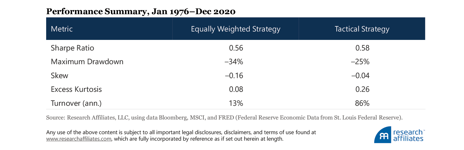
In the extended backtest, the tactical strategy provided higher cumulative returns and better drawdown characteristics (maximum drawdown of −25% versus −34%) versus the equally weighted benchmark. The risk-adjusted return, or Sharpe ratio, of the TAA strategy is only marginally better (0.58) than the Sharpe ratio of the benchmark (0.56).
Why does the tactical strategy’s outperformance decrease relative to the benchmark when we extend the backtest to 1976? We examined the portfolios decade by decade and observed that for the periods prior to the original backtest, the tactical strategy meaningfully underperformed the equally weighted benchmark, particularly in the latter half of the 1970s (0.32 versus 0.59).
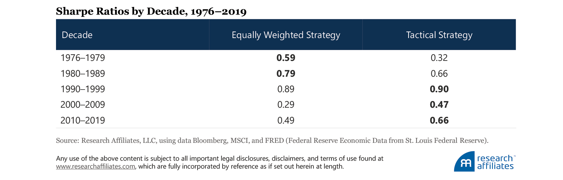
Under our macroeconomic framework, the period from 1976 to 1979 was forecasted as having decelerating inflation when measured against the high-inflation trend observed through the first half of the 1970s. Compounded by the fact that the S&P GSCI was heavily biased toward its oil components, an underweight in commodities (as oil prices spiked in late 1970s) as governed by the TAA strategy was particularly detrimental in the years before 1979. This tilt resulted in a significant decrease in the TAA strategy’s Sharpe ratio versus the benchmark.
Please read our disclosures concurrent with this publication: https://www.researchaffiliates.com/legal/disclosures#investment-adviser-disclosure-and-disclaimers.

Endnotes
- We certainly are not the first to use growth and inflation as indicators of the business cycle; for example, growth and inflation form the core of the Bridgewater All Weather investment strategy (Bridgewater, 2012). Additionally, we are not implying that growth and inflation are the only two indicators an investor should consider to model the business cycle.
In many of our TAA strategies, we do employ alternative methods that construct proprietary indices meant to forecast where the business cycle will be in the coming three to six months. Those signals can at times differ from the simple approach presented here.
- The high inflation of the 1970s is not our expectation for the future. Consequently, our focus in this analysis is on inflation shocks and surprises. We acknowledge our results would be different had we focused on the level of inflation. We provide extended results of our portfolio analyses back to 1970 in the appendix.
References
Ang, Andrew. 2014. Asset Management: A Systematic Approach to Factor Investing. Oxford University Press: New York, NY.
Attié, Alexander, and Shaun Roache. 2009. “Inflation Hedging for Long-Term Investors.” IMF Working Paper No. 09/90 (April 1).
Bodie, Zvie. 1976. “Common Stocks as a Hedge Against Inflation” Journal of Finance, vol. 31, no. 2 (May):459–470.
Bridgewater Associates. 2012. “The All Weather Story.” Bridgewater.com (January).
Fama, Eugene, and G. William Schwert. 1977. “Asset Returns and Inflation.” Journal of Financial Economics, vol. 5, no. 2 (November):115–146.
Kritzman, Mark, and Yuanzhen Li. 2010. “Skulls, Financial Turbulance, and Risk Management.” Financial Analysts Journal, vol.66, no. 5 (September/October):30–41.
Levine, Ari, Yao Hua Ooi, and Matthew Richardson. 2016. “Commodities for the Long Run.” NBER Working Paper 22793 (November).
