
The risks of factor investing are usually understated (perhaps, severely so), and the diversification benefits tend to be overstated.
Because factor returns substantially deviate from normality and because correlations between factors are not constant over time, a multi-factor portfolio may retain exposure to the risk drivers of the individual factors. Thus, portfolios invested in multiple factors may still experience severe drawdowns and decade-long periods of underperformance.
Factor investing, for patient investors who understand the risks, has the potential to improve a portfolio’s long-term risk-adjusted return, especially when strategies used are transparent, use sufficiently researched factors, and have low management fees and good implementation characteristics.
Factor investing, an investment approach which targets specific stock characteristics such as value or momentum, is becoming a stronghold of investor portfolios.1 Many factor-investing strategies are popular for good reason: they are transparent, offer exposure to widely agreed-upon sources of expected return, have low management costs and, with proper design, reasonable transaction costs. Of course not all products in the category provide all of these features. When these features are present in a strategy, however, the strategy has the potential to generate a substantial positive impact on investor returns.
Product providers blithely advertise the benefits of factor investing, touting the strong long-run (usually backtested) value-add of individual factors, the manageable tracking error, and the low average correlations of most individual factors. The usual factor-investing sales presentation leaves an impression that investing in factors means almost guaranteed excess returns and that investing in a number of factors eliminates most of the risks of underperformance as a result of diversification. The standard disclaimer that follows the presentation cautions past performance is not indicative of future returns, the excess return is not guaranteed, and so forth, while offering little information about the specific dangers of factor investing. The combination of positive messaging in presentations with easily overlooked or disregarded disclosures means that investors too often ignore, and thus do not prepare for, the risks that come with factor investing.
Not fully understanding the myriad risks that lie ahead in the investment journey, investors are likely to make poor choices about when to begin and end their investment in a particular strategy. Entering at the wrong time, or missing a few market turning points, can mean the investor is ultimately a net loser in factor investing. Factor investing can be a very useful tool, however, to help investors enhance their return and make prudent investment choices if they do so with full knowledge of the strategy’s potential risks.
Risks of Factor Investing
Factors definitely have risks, and ignoring these risks can leave investors hugely underprepared for the investment journey. Investors, for example, can have difficulty understanding how the average value-add and tracking error of a factor translate into underperformance, a very practical concern for many investors.2 Another wrinkle is that the return distributions of most factors substantially deviate from the normal distribution, so that large outlier returns appear far more frequently than investors might expect. Further, some factor returns may be serially correlated; that is, future returns are not independent of past returns.3 For factors, poor performance may likely be followed by further periods of poor performance, and such continuation can make periods of underperformance excruciatingly painful.
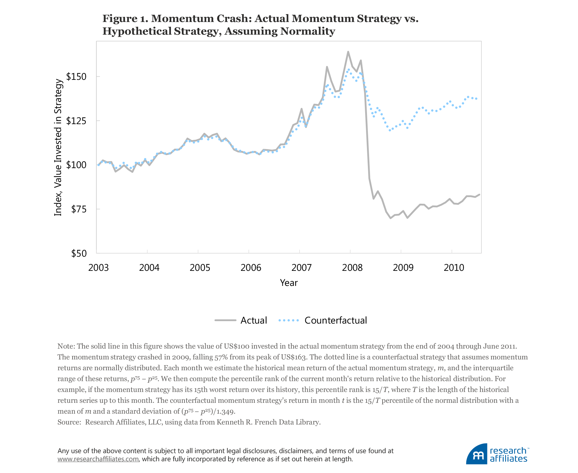
We can take a look at the momentum strategy, for example, to gain a better understanding of the risks involved. Figure 1 compares the realized performance of a long–short momentum portfolio with a counterfactual momentum strategy in which returns are calibrated to be normally distributed. The trend in both strategies from the beginning of 2005 through March 2009 was positive, but that changed in the following month. For the month of April 2009, the momentum trade returned −36%, the strategy’s worst month since January 1963. In the calibrated normal distribution, however, this percentile of realized performance would have equated to a return of −8%. An investor who had assumed returns are normally distributed would never have foreseen that the strategy’s return could be as extremely negative as it turned out to be.
Finally, and perhaps most dangerous of all, factor investing presents the risk of data mining. Only factors that show good backtest results are published, let alone used. The resulting upward bias in return estimates is known as selection bias. A factor may look good because it is good or because the historical record is randomly good. Because disentangling the two can be a difficult proposition, the historical results should be expected to exceed future efficacy. In some cases, historical data can even create an illusion of value added by a strategy which in reality has no structural efficacy (Harvey, Liu, and Zhu, 2016). Similarly, the backtest results that attract investors and their capital were mostly earned during a span when little money was being committed to these factor-tilt strategies. An influx of capital can easily arbitrage away the efficacy of a factor, and in some cases this may already have happened for certain factors (McLean and Pontiff, 2016).
Introducing the Factors
The usual list of factors presented to investors includes value, momentum, low beta, size, and quality. Although hundreds of characteristics that appear to show statistical significance in a historical realization have been documented in top-tier academic journals, many of these purported factors may simply result from data mining, uncovering random regularity. Several studies, such as Harvey, Liu, and Zhu (2016) and Beck et al. (2016), provide an examination of the wide roster of factors and narrow down the list to a few having the strongest evidence of producing an historical premium.4
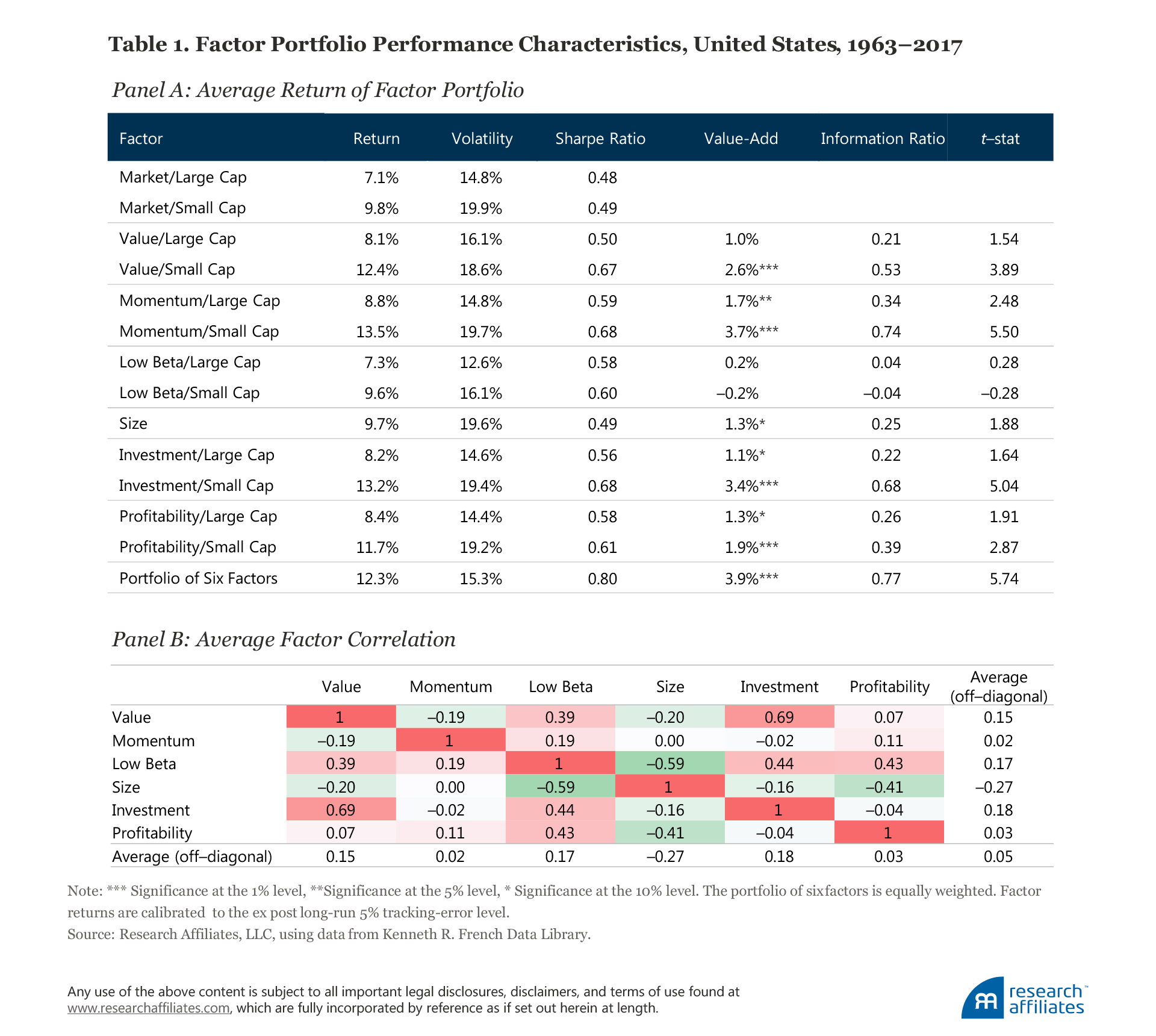
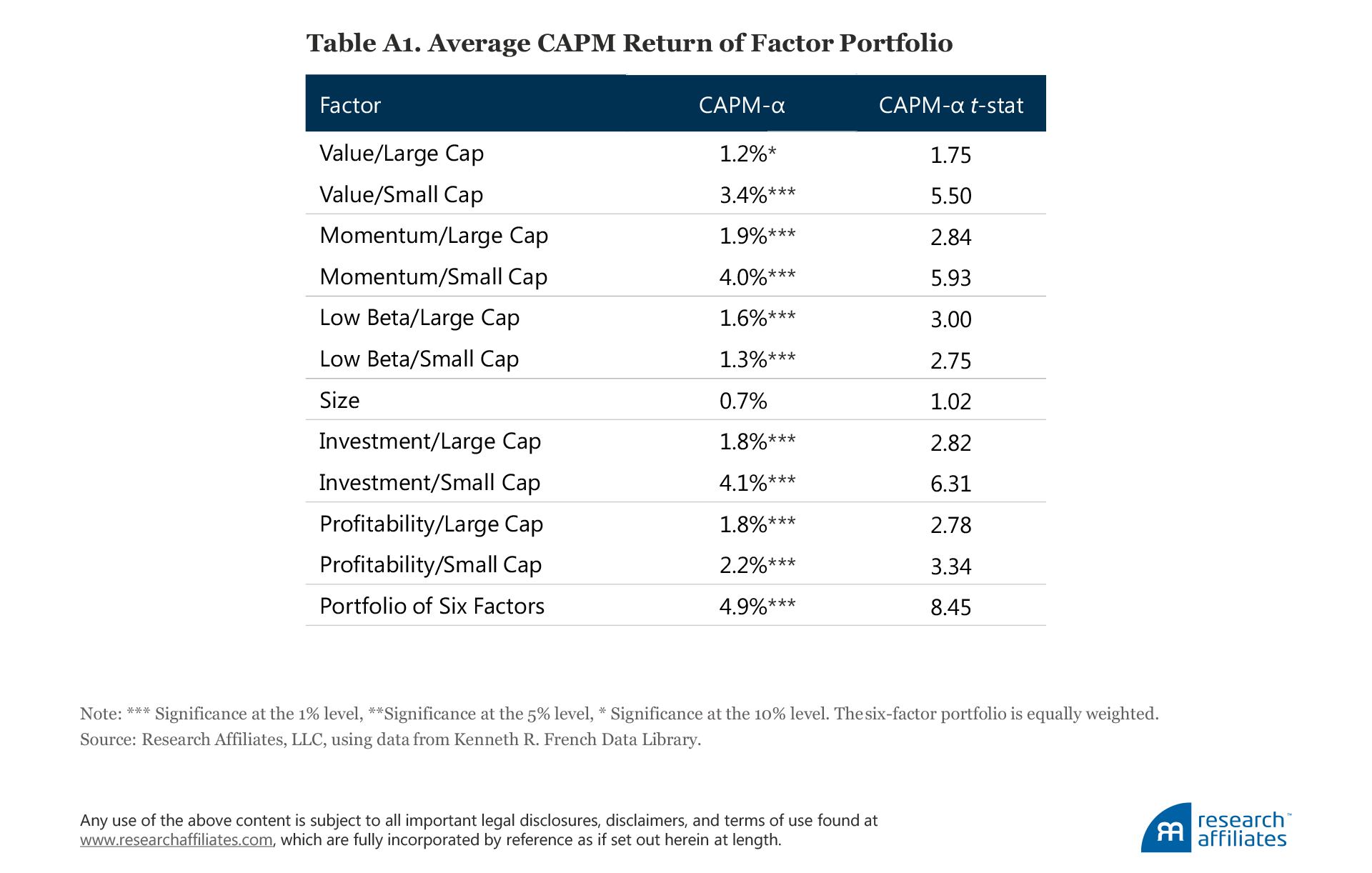
Table 1 reports the long-run average returns and correlation characteristics that investors commonly study when they examine factors. We define a factor’s value-add as the average return on a long–short factor that is standardized to have an annualized volatility of 5% a year.5 The first three columns in Table 1 consider long-only portfolios, which we construct by overlaying these 5% long–short factors on top of the market portfolio. (We provide the simulation details for all tables in the appendix. We also report the CAPM alphas for these portfolios and their t-statistics in Table A1 of the appendix.) The 5% volatility standardization means therefore that each factor’s tracking error is 5%. Let’s begin our discussion with a few basic facts about the following five common factors:
- The value factor favors stocks that have lower price-to-fundamentals ratios, such as price to book, price to earnings, and price to dividends, going long these stocks, while selling short those stocks that have higher price-to-fundamentals ratios. Basu (1983) first documented in the academic literature that stocks with value characteristics have superior performance. As shown in Table 1, Panel A, the value premium has been historically strongest among small stocks. The persistence of the value premium has been explained in two different ways: 1) the risk-based explanation argues that value stocks are more risky and are possibly linked to undiversifiable permanent shocks to consumption, whereas 2) the mispricing explanation suggests that stocks can be mispriced for behavioral reasons and that limits to arbitrage, such as a short-term evaluation horizon for managers, limited access to credit, and costly shorting, prevent arbitrageurs from pushing prices toward fundamental values.6
- The momentum factor invests in assets with high returns over a certain formation period, which typically ranges from six months to a year, and sells short assets with low returns over the same time period. The momentum factor therefore bets on return continuation, relying on the regularity that high returns are typically followed by high returns and that low returns are typically followed by low returns. Jegadeesh and Titman (1993) first documented the momentum premium. Table 1, Panel A, shows that the momentum trade has historically been profitable—significantly more so among small stocks. Most explanations for the persistence of the momentum premium rely on the initial underreaction of a stock’s price to news due to limited attention in the marketplace.7
- The low-beta factor favors low-beta stocks. Black, Jensen, and Scholes (1972) and Haugen and Heins (1975) documented that stocks with a higher beta do not produce meaningfully higher returns than low-beta stocks. As a consequence, on a risk-adjusted basis, low-beta stocks significantly outperform high-beta stocks (Black, 1993). Because market beta is the main driver of the risk of a diversified equity portfolio, investing in a portfolio of low-beta stocks provides significantly more attractive risk–return characteristics, which shows up as a very high Sharpe ratio in Table 1 despite unimpressive value-add, and also as statistically significant CAPM alpha as reported in Table A1 of the appendix.8 The low-beta effect has been explained by 1) the presence of leverage constraints so that investors tend to use high-beta stocks to increase portfolio returns (Frazzini and Pedersen, 2014) and 2) the use of high-beta stocks for speculation or as substitutes to lotteries.
- The size factor was first documented by Banz (1981) when he found that stocks with small market capitalizations tended to outperform stocks with large market capitalizations. Our findings reported in Table 1, Panel A, show the same results. In order to capture the small size premium, the size factor favors small stocks. Explanations for the small-size premium include: 1) small stocks may be younger with greater growth potential and may also expose investors to an undiversifiable, potentially distress-related risk because small companies are more capital constrained (Fama and French, 1993); 2) a significant portion of the small-cap premium computed by researchers may be a data mistake caused by the improper treatment of the delisting returns of stocks (Shumway, 1997, and Shumway and Warther, 1999); and 3) a near-mechanical link between expected returns and size, so that if two firms have identical expected cash flows but one has a higher expected return, the smaller-sized firm will have the higher expected return.9
- The quality factor favors the stocks of companies that exhibit some measure of higher quality in their financial characteristics. Reasons given for the quality effect include: 1) a risk-based explanation, proposed by Hou, Xue, and Zhang (2015), that argues riskier companies, which face a higher cost of capital in the equilibrium, should have higher profitability and lower rates of investment; and 2) a mispricing explanation that argues companies with higher profitability and low investment are conservative businesses, which have strong moats to protect their profit margins and which also stay out of the glamour spot light, ensuring that investors do not overpay for the cash-flow distributions of these companies. In an examination of quality-related investing, Hsu, Kalesnik, and Kose (2017) found that the quality factor combines a number of anomalies associated with strong business entities. Their survey shows that multiple factors commonly used in the practitioner community as a proxy for quality, including leverage and earnings growth, lack strong evidence of producing a quality premium. Stronger evidence of a systematic premium was demonstrated when quality was defined as investment, profitability, equity issuance, and accounting quality; of these four, profitability and investment, included in Table 1, Panel A, have the most acceptance in the academic literature.
Each of these factors has an Achilles’ heel, giving rise to serious concerns about its future efficacy. For value, it’s the two 11-year bear markets—the most recent from August 2007 to today—that the factor has experienced, which begs the question: Is the value insight today permanently impaired or still indicative of truly cheap stocks? We believe the latter, but cannot prove it. Momentum’s long-term track record would be truly brilliant in the absence of trading costs, but turnover is huge, and trading costs can devour the alpha. Standard momentum, defined as trailing year excluding the latest month, has lost more since 1999 in its crashes than it has earned in its bull markets. Nevertheless, in defense of both value and momentum, these two effects have existed across multiple asset classes (Asness, Moskowitz, and Pedersen, 2013) and, in the case of momentum, for over two centuries (Geczy and Samonov, 2016). Are these two effects now gone, forever, in all their forms?
The size factor, despite being one of the first factors identified, offers very weak empirical evidence of a long-run premium. The performance of the investment factor, which is considered part of quality, is very sensitive to its definition (Cooper, Gulen, and Ion, 2017), raising potential concerns around data mining. Low beta faces the existential question: Should a low-risk portfolio perform on par with, or even better than, a high-risk portfolio? The leverage-constraint explanation for the low-beta effect only works if these constraints remain important. Moreover, Arnott, Beck, and Kalesnik (2016a,b) suggest a portion of the alpha earned by the low-beta factor so far this century is attributable to its rise in “relative valuation”: low-beta stocks used to trade at a deep discount, but now trade at a substantial premium.
These factors’ Achilles’ heels do not mean that factor investing is a mistake. We would simply encourage investors to acknowledge that any of these factors may be periodically structurally impaired, unable to produce reliable positive alpha in the years ahead. By investing in multiple factors, however, investors can improve the odds of benefiting from those factors that are able to generate excess returns in the coming years.
By investing in multiple factors, diversification can mitigate the risks of individual factors, reducing a portfolio’s overall risk—but far from all of it. Long-run low correlations can mask the time-varying nature of factor correlations and potentially some of the underlying systematic components of factor performance. Especially during crises, previously minimally or negatively correlated assets can become positively correlated, destroying in the short run the benefits of diversification. Combinations of factors, just like individual factors, also experience lengthy and sizeable drawdowns.
Some product providers are quick to show a correlation matrix with very low, and sometimes negative, values to suggest that diversification benefits remove almost all of the risk associated with individual factors. The commonly presented evidence for factor returns tends to imply that factor returns are typically almost normally distributed and serially uncorrelated, suggesting large losses are very improbable. Also, a correlation matrix of the value-add of different factors, as shown in Table 1, Panel B, can lead investors to the conclusion that most factors are almost uncorrelated—the average off-diagonal correlation of the six factors is 0.05 (the average of absolute off-diagonal correlations is 0.22, which is also quite low). Investors can erroneously conclude that by investing in multiple factors they will be able to eliminate through diversification almost all of the risk associated with individual factors.
Factor Drawdowns When Everything’s “Normal”
The average return and volatility of long–short factors and the value-add, volatility, and tracking error of long-only factors are just abstract characterizations of a factor’s performance and require some translation into the tangible characteristics of return and risk that investors care about. In practice, investors want to know about two types of risk: 1) absolute return and 2) return relative to a benchmark or peer group. Absolute performance is extremely important because it produces the absolute wealth available to an investor.
The relative return is no less important—and will be the focus of our discussion here. Not only does a long period of underperformance relative to the investor’s benchmark mean the asset manager is likely to be fired, it also perpetuates a cycle in which the investor sells recent losers and buys recent winners. Consequently, caught in this cycle the investor will routinely underperform from poor timing decisions. Russel Kinnel (2005), and many after him, documented that investors’ realized returns are, on average, 200 basis points a year lower than the buy-and-hold returns of the same underlying funds.10 Arnott, Kalesnik, and Wu (2018, forthcoming) provide evidence that the return gap is largely driven by investors selling funds after periods of poor performance, (i.e., selling newly cheap assets), and buying funds after they have performed well (i.e., buying newly expensive assets).
Practically speaking, investors are very sensitive to drawdowns relative to a benchmark portfolio and to sustained periods of underperformance in which they spend years or even decades below the previous high point; the longer and deeper in magnitude these episodes are, the more likely they will translate into negative consequences for the agents overseeing the portfolio (they are fired) or for the investor, who makes a poor timing decision in fund rotation.
We will begin by examining drawdown periods of relative performance, assuming factor returns are “well-behaved” (i.e., that very extreme return realizations are unlikely). Mathematically we can approximate this behavior by using a normal distribution of returns. Many day-to-day phenomena are normally distributed, thereby informing our understanding of randomness. For example, the height and weight of the majority of the population are more or less normally distributed and do not deviate much from the average. Whereas we routinely observe values that deviate from the average, we rarely, if ever, observe “true” outliers that are more than four or five standard deviations from the average.
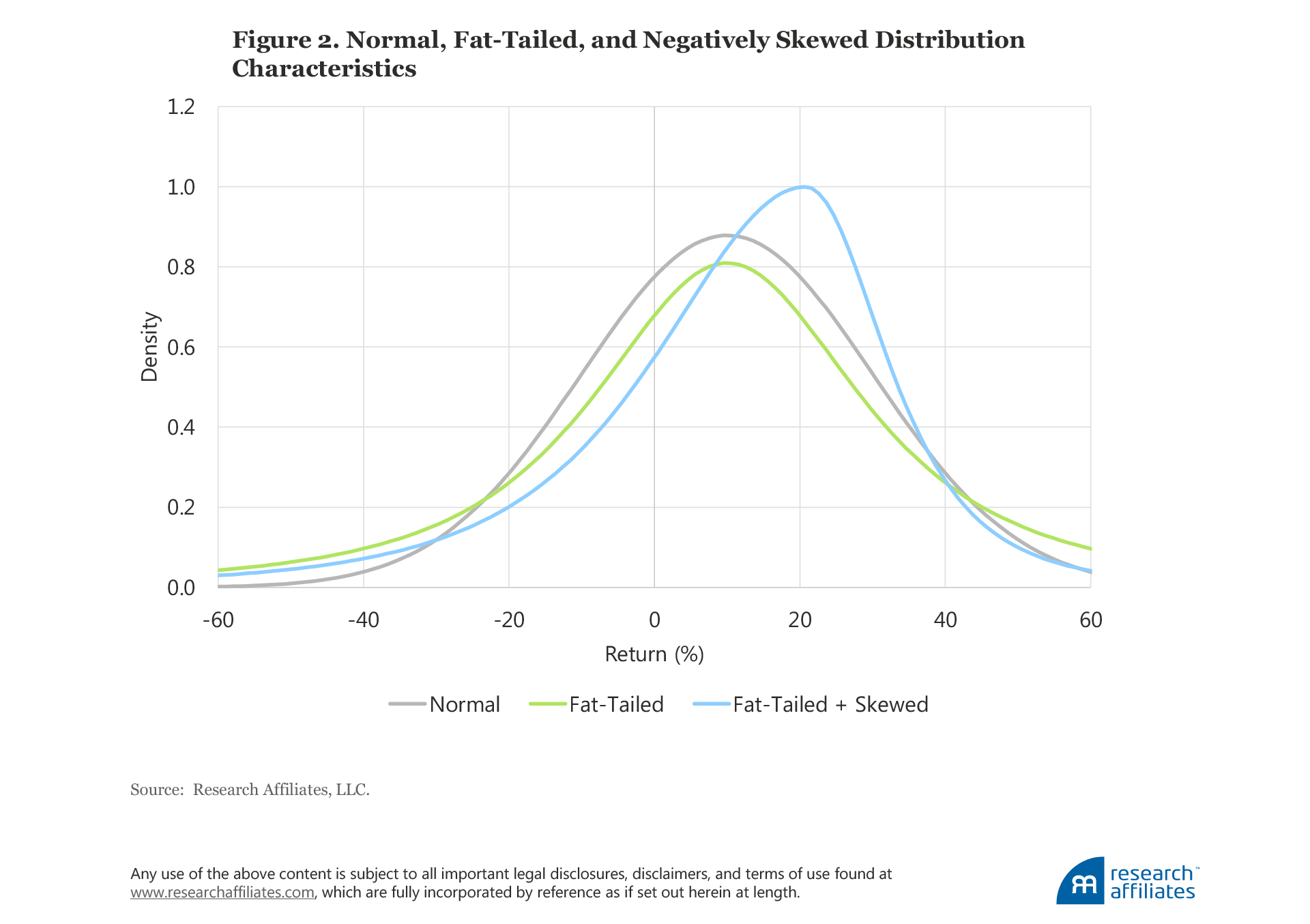
A distribution is characterized by a density function which indicates the likelihood of observing a realization of a given magnitude. The gray line in Figure 2 shows the density function of a hypothetical normally distributed variable with a 10% average return and 20% standard deviation. Under normality, the realizations are symmetric around a 10% return; extreme realizations, below a –50% return and above a 70% return, very quickly become unlikely. Figure 2 also shows the hypothetical distributions for a fat-tailed scenario (green line) and a negatively skewed scenario (blue line). They have the same average and standard deviation of returns as the normal distribution, but both have a higher likelihood of observing extreme realizations. Occurrences of both extreme positive and extreme negative outliers are much more likely for the random variable following the fat-tailed distribution, and extreme negative outliers are much more likely for the negatively skewed distribution.
In Table 2, we characterize the drawdown characteristics of six factors assuming the returns are normally distributed.11 Factors are typically constructed using a long–short portfolio. The majority of investors, however, invest in long-only strategies. Fortunately, this difference is easy to resolve. In the long-only setting, the average factor return roughly translates into the average value-add, and the volatility roughly translates into the tracking error. To make our drawdown estimates as applicable as possible, similar to the simulation just presented, we calibrate to the ex post long-run 5% tracking-error level. We characterize drawdowns in a typical 55-year experience of investors’ allocating to various factors by assuming the factor return is normally distributed and calibrated using the average return and volatility.12
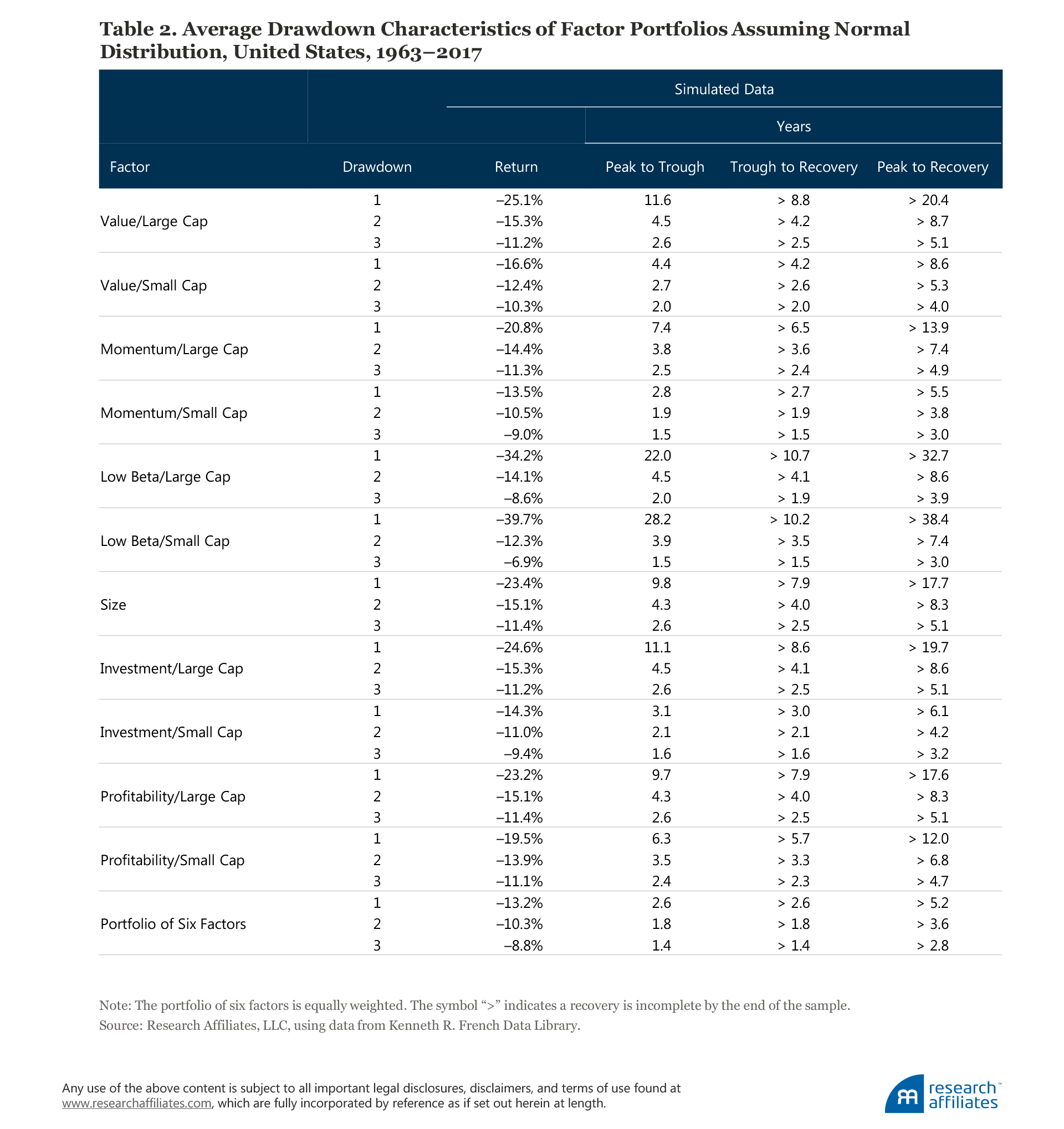
In Table 2 we display the average characteristics of the first-, second-, and third-largest drawdowns from multiple simulations for each factor. We display the average return at the bottom of the drawdown as well as the length of this drawdown. Because we simulate finite 55-year sample periods, a recovery can be incomplete by the end of our sample. We therefore mark years to recovery with “>”.
For value defined in the large-cap space (e.g., Value/Large Cap in Table 2), the average worst drawdown over the 55-year span is 25.1%.13 The typical time spent from the previous peak to trough is 11.6 years, and it takes at least 8.8 years to recover. The total time spent below the previous peak is more than 20 years.14 For practical purposes, this result indicates that the typical value investor should expect to spend about a decade underperforming the benchmark in a typical 55-year investor experience.
For the factors defined within the large-cap universe (plus the size factor), the typical worst drawdown experienced in a 55-year span tends to be about 25%, and for Low Beta/Large Cap is as high as 34%. Investor portfolios invested in these factors tend to spend about 20 years below the previous peak. This average is quite close to the experience for the value factor. For factors defined within the small-cap universe, the average worst underperformance is 21%, although the range is wide, from 13.5% for Momentum/Small Cap to 39.7% for Low Beta/Small Cap. The average time an investor’s portfolio spends below the previous peak is 14 years, which is better than for factors defined in the large-cap space, but still quite scary.
The worst factor drawdowns in a typical 55-year investor experience can be quite daunting, however, the average second- and third-largest drawdowns are also quite bad. For large-cap factors, the average second- and third-worst drawdowns are 15% and 11%, respectively, with the average time from peak to recovery being 8 and 5 years, respectively. For factors defined in the small-cap universe, the drawdowns are 12% and 9%, respectively, and the times from peak to recovery are 6 and 4 years, respectively.
When we combine these factors in a portfolio, the drawdowns become significantly milder in magnitude and the length of underperformance considerably shortens. The worst drawdown is 13.2%—about half the 23% average drawdown experienced by the individual factors defined within both large-cap and small-cap universes—with a time from peak to recovery of 5.2 years, about a quarter of the 18 years for the individual factors. The second- and third-worst drawdowns, at 10.3% and 8.8%, respectively, also are milder in magnitude and at 3.6 and 2.8 years, respectively, quite short in length. Diversification certainly helps in this theoretical case.
“Normality” Faces Reality
The reality is that factor returns are far from normally distributed. The assumption of a normal distribution and no serial correlation greatly underestimates the occurrences of extreme outcomes. To illustrate this point, we report in Table 3 the worst monthly factor return realizations in the US market over the last 55 years for the six strategies and the equally weighted six-factor portfolio, targeting a 5% tracking error.15 We report estimates of how frequently we should expect losses of this magnitude if we were to assume that returns are normally distributed. Of the dozen extreme observations, 10 should have occurred less frequently than at least once during the length of the recorded history of mankind, 6 should have occurred less frequently than the length of the period biologically modern humans have roamed the earth, and 3 should have occurred less frequently than since our universe was created as the result of the Big Bang about 13.8 billion years ago.
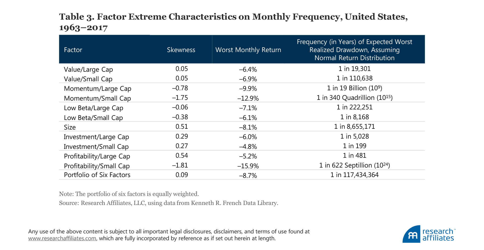
If we assume normality for the diversified portfolio of six factors, we would have observed the worst realized monthly return of 7.9% only about once every 117 million years, or only once since the Tyrannosaurus Rex and Velociraptor ruled our world—yet we have lived through this extreme realization in just the last 55 years.
To make things worse, factor returns can be serially correlated. Arnott et al. (2018) and Ehsani and Linnainmaa (2018) show that factors with high recent performance continue to outperform factors with poor recent performance. This momentum effect in factor returns can make the periods of underperformance even more painful when poor performance is followed by yet more poor performance.
In the previous section, we described the drawdowns we would expect to observe given the assumption of a normal distribution of returns and the assumption that the returns in one period are independent of past returns. Now let’s compare past realized drawdowns with theoretical drawdowns across the equity markets of the United States, Europe, the developed nations, and Asia Pacific excluding Japan.
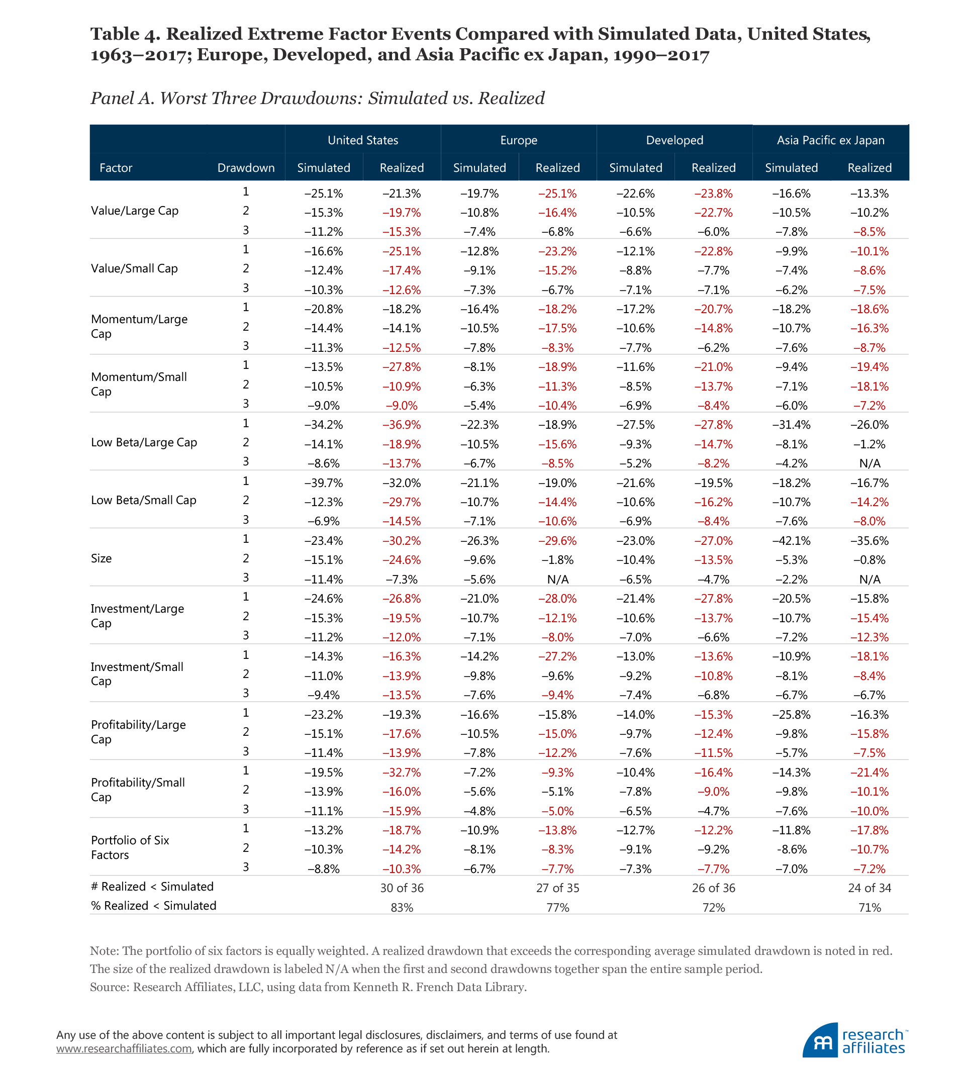
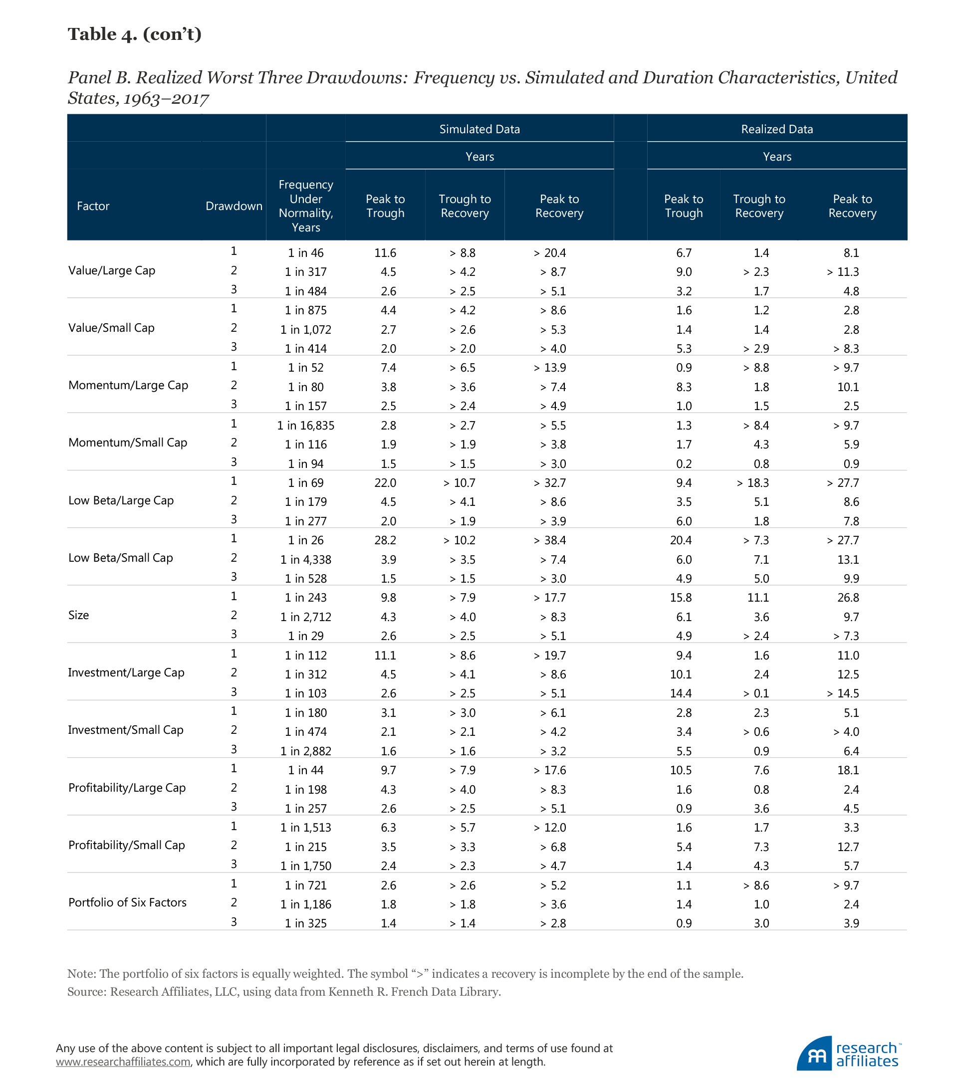
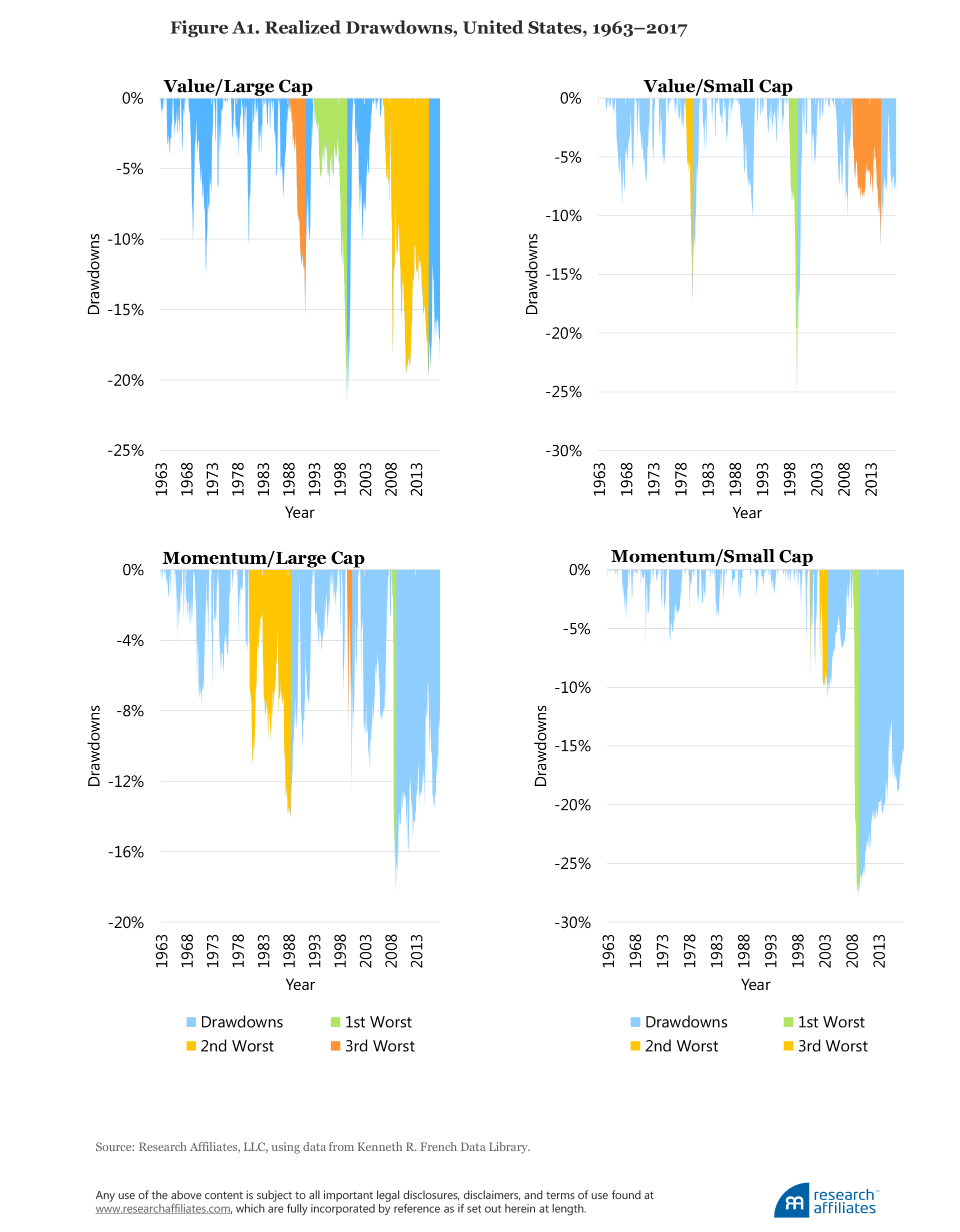
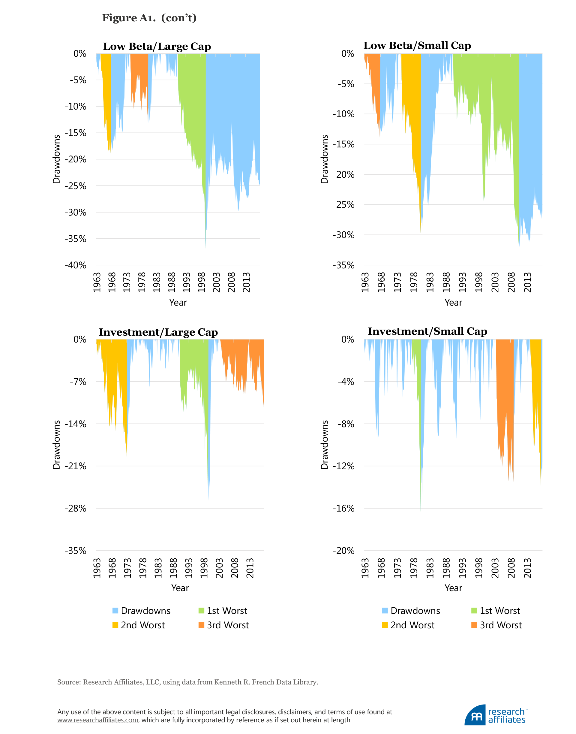
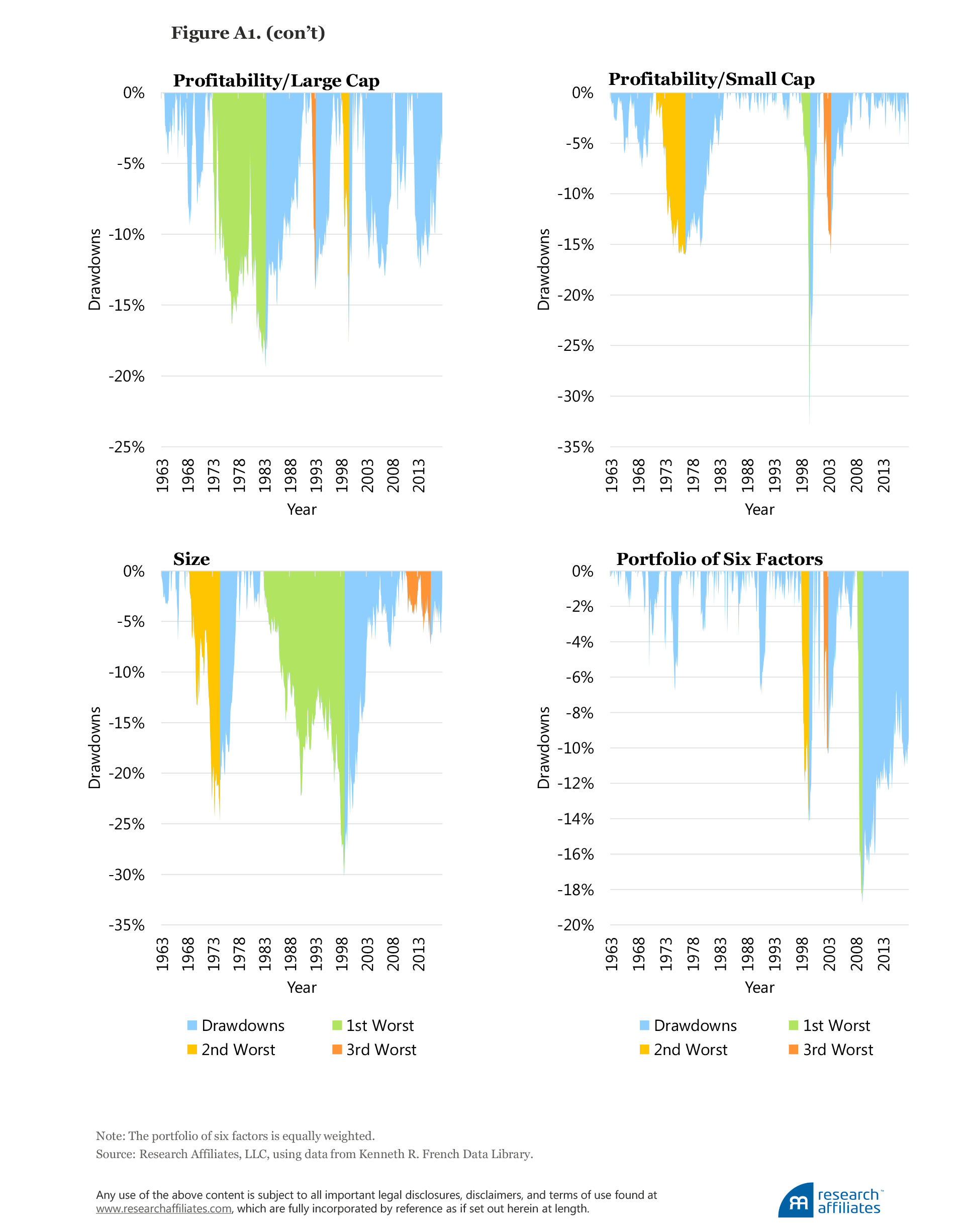
We report in Table 4, Panel A, the magnitude of the worst three realized drawdowns for each of the six factors in our analysis as well as for the portfolio of six factors over the last 55 years in the United States and over the last 28 years, 1990–2017, in Europe, Developed Markets, and Asia Pacific excluding Japan. We indicate in red each realized drawdown that exceeds the corresponding average simulated drawdown. In Table 4, Panel B, we also report for the longer US sample the duration characteristics and frequency at which we would expect to observe an event of this magnitude if returns were normally distributed and not serially correlated. We provide the details of the estimation in the appendix along with graphic illustrations of realized drawdowns for the six factors over the 1963–2017 period in the US market.
We observe the following from our analysis, based on the US market data:
- In 83% of realized drawdowns, the magnitude of drawdown is more severe than would have been expected if returns were normally distributed. In the shorter international samples, realized drawdowns were worse in 70% to 79% of cases. Realized drawdowns were, on average, worse than simulated drawdowns for all factors without exception.
- For the value factor, the duration of the drawdown (from performance peak to trough) tends to be on par with what we expect under normality. The recovery, however, tends to be quite sharp, usually as the market bubble bursts, which differs from our expectation under normality.
- When the momentum factor is defined within the small-cap universe, we observe some of the most extreme differences between realized and simulated performance. Under normality, we would expect to observe a drawdown of 27.8% only once every 17,000 years, a period so long that, to go back that far, much of the planet would have been in the midst of the Ice Age. For the momentum factor, in general, the time from previous peak to trough is substantially shorter than what we should expect under normality because of momentum’s tendency to experience sharp crashes.
- The low-beta factor, defined within both the large- and small-cap universes, exhibits the greatest magnitude of underperformance of all factors. As we noted earlier, the low-beta factor does not earn a positive risk premium before we control for market risk. This means that low-beta strategies can underperform the market portfolio for long periods of time. The shrewd reader will recognize we are dealing with a benchmark-mismatch problem; that is, the market portfolio is not the appropriate benchmark for the low-beta portfolio, because the benefit of the low-beta portfolio is in risk reduction and not in delivering value-add over the market portfolio. A low-beta portfolio earns an average return comparable to that of the market, and its benefit comes from the fact that it assumes less market risk.
- Diversification does reduce risk, but far from completely. The realized drawdown characteristics of the six-factor portfolio are disappointing compared to the simulations. In the US market simulation, the worst drawdown was 13.2%, with the period from peak to recovery extending a little over five years. The realized worst drawdown in the United States over the last 55 years was 18.7%—and still we have not reached the last peak observed almost a decade ago. Even the second-worst realized drawdown of 14.2% is more severe than the 13.2% worst drawdown under the assumption of normality. This observation drives home the point that if we assume correlations are constant, and that we can diversify away almost all factor risk by investing in multiple factors, we may be in for an unpleasant surprise. Investors in the last quant crash, who were assuming low correlations among investment assets, can bear witness to the cost of such an assumption.
In summary, realized periods of underperformance when compared to underperformance estimated by theoretical normally distributed data show 1) more severe drawdowns; 2) for value factors, quite prolonged periods from peak to trough often followed by speedy recoveries; 3) sharp momentum crashes, and 4) limited diversification benefits from combining factors into portfolios.
Conclusion
Factor investing is gaining popularity. Many academic articles and presentations to practitioners make a convincing case that factor investing will likely generate premia for investors who are willing to take factor exposure. Unfortunately, the risks of factor investing are usually understated (perhaps, severely so) and the diversification benefits tend to be overstated. Investors who underestimate the risks associated with factors, and who expect more reliable alpha than is plausible with factor investing, may well be disappointed in their performance and switch strategies at the wrong time, lessening the likelihood they will make their long-term return targets.
Individual factors are likely to experience lengthy and severe drawdowns, and diversification across factors cannot be expected to eliminate all the risks of factor investing—even though frequently cited low historical correlations, especially derived from backtests, can be very impressive. The reality is that correlations between factors are not constant over time and multiple factors may be exposed to the same underlying risk drivers. Thus, investors with exposure to multiple factors may still experience severe drawdowns and decade-long periods of underperformance.
We believe the attraction of factor investing is partly, and perhaps even largely, fueled by investors seeking to move away from value-oriented strategies after a decade-plus period of underperformance in order to seek what they believe will be a more reliable source of return. Low beta and momentum also experience very long periods of underperformance relative to the benchmark, and have considerably large drawdowns, but with their historically low correlations to value are value’s natural complements, serving to lower portfolio risk when the factors are combined. This benefit is a major part of their appeal to value investors.
Simply put, in the right hands, given appropriately tempered expectations, and used by investors prepared to weather potential periods of material underperformance, long-only factor investing, often called smart beta, can be a valuable way for investors to achieve their long-term return targets.
Appendix
Computational Details
Figure 1 tracks the value of $100 invested in the actual and counterfactual momentum strategies from the end of 2004 through June 2011. The return on the actual momentum strategy is the UMD factor (Carhart, 1997), which is an equally weighted combination of Momentum/Large Cap and Momentum/Small Cap. We assume that the investor rebalances the long and short legs each month, and therefore his wealth W in month t + 1 is Wt+1 = Wt × (1 + UMDt+1). The counterfactual momentum strategy replaces actual momentum returns with those drawn from a calibrated normal distribution. Each month we use historical data from July 1963 through month t to compute the average monthly UMD return and its interquartile range p75 – p25. We compute the return on the counterfactual momentum strategy based on these statistics. Using the historical distribution of realized UMD returns, we first compute where the month t + 1 return falls on this distribution. For example, if the UMD return is the 15th worst return realization based on T months of historical data, this return realization’s percentile rank is 15/T. We then draw from the calibrated normal distribution the return that corresponds to this percentile.
Table 1 reports average returns, volatilities, value-adds, information ratios, and t-values for the market, six factors, and an equally weighted portfolio of the six factors. Market/Large Cap and Market/Small Cap are computed using the six portfolios sorted by size and book-to-market ratio. Market/Large Cap is the average return on the big-value, big-neutral, and big-growth stocks. Market/Small Cap is the average return on the small-value, small-neutral, and small-growth stocks. These same definitions are used for the size factor, SMB (Fama and French, 1992). The value, momentum, size, investment, and profitability factors are computed using data on the six portfolios sorted by size, and alternatively by book-to-market ratio (value), prior one-year return skipping a month (momentum), book-to-market ratio (size), year-to-year growth in total assets (investment), and operating profitability (profitability). The large-cap factor is typically the return on the high big-stock portfolio minus the return on the low big-stock portfolio; the investment factor reverses these assignments. The small-cap factor is defined the same way using the small-stock portfolios. Size is the average return on the three small-cap portfolios minus the average return on the three large-cap portfolios. The low-beta factor is constructed using data on the 25 portfolios sorted by size and market beta. We define the small low-beta portfolio as the average return on the four portfolios in the small low-beta corner of these 25 portfolios; the other portfolios are similarly defined as the average return on the four corner portfolios in the other three corners. We then define the Low Beta/Large Cap and Low Beta/Small Cap portfolios as the differences in returns of these average corner portfolios. The return of the equally weighted portfolio of six factors is the average return of the six factors. Before taking this average, we define value as the average of the Value/Large Cap and Value/Small Cap; momentum as the average of Momentum/Large Cap and Momentum/Small Cap; and so forth. We standardize each long–short factor to have a full-sample annualized standard deviation of 5%. The first three columns in Panel A, labeled “Return,” “Volatility,” and “Sharpe Ratio,” overlay each factor with the market portfolio of the corresponding size. The return on Value/Large Cap, for example, is the return on the large-cap market portfolio plus the large-cap value factor standardized to 5% volatility. The estimates in the other columns, beginning with “Value Add,” report the statistics for the factors standardized to 5% volatility without the market overlay. The correlations in Panel B are similarly based on the long–short factors without the market overlay.
Figure 2 illustrates the differences between returns that are normally distributed and those that follow either fat-tailed or fat-tailed and skewed distributions. Each distribution has a mean of 10% and a standard deviation of 20%. The fat-tailed distribution is t-distributed with two degrees of freedom. The fat-tailed and skewed distribution is a generalized skewed t-distribution with λ = –0.3, p = 2, and q = 1.5.
Table 2 describes the average characteristics of the three largest drawdowns in a 55-year sample when factor returns are normally distributed. For each factor, we draw returns from a normal distribution that has the same mean and standard deviation as the average factor returns and the standard deviation from July 1963 through May 2018. We generate 500,000 samples, each with a length of 660 months, and then determine the largest three drawdowns in each sample. We report the average size of each drawdown and the time it takes, in years, to reach the trough, or to recover from the trough. Because the recovery can be incomplete by the time a 55-year sample ends, we mark the times from trough to recovery and from peak to recovery with a “>” to indicate these estimates are based on truncated data.
Table 3 reports how likely it would be to observe a monthly factor return that would be as negative as the worst realization from July 1963 through May 2018. We first define t-statistic = (Worst monthly return realization − Average monthly return) / Standard deviation of monthly returns. We then compute the percentile in the normal distribution that corresponds to this t-value and report the frequency based on this percentile. A t-value of –1.96, for example, corresponds to a percentile of 0.025, which means we would expect to observe a return of this magnitude (or worse) once every 40 months, or every 3.33 years.
Table 4 uses the same factors as Tables 1 through 3 except that, in addition to the United States, we also report the same statistics for Europe, Developed Markets, and Asia Pacific excluding Japan. All factor data, except for the low-beta factor in each of these additional markets, are from the Kenneth R. French Factor Library. The low-beta factor is computed using data from Thomson Reuters Datastream. We first estimate betas at the end of each month using one year of daily data. We then assign stocks into small and big groups based on market capitalization and then, conditional on size, we assign stocks into low-, medium-, and high-beta categories. The return on the beta factor is the average return on the value-weighted low-beta portfolio minus the average return on the value-weighted high-beta portfolio.
Endnotes
1. At the end of 2017, funds categorized by Morningstar Direct data as strategic beta funds held about US$767 billion in assets under management. This amount represented an annualized increase of about 20% over the previous five years.
2. Barberis and Thaler (2003) and Barber and Odean (2013), among others, survey the literature on investor behavior and discuss the biases and cognitive limitations that hinder investor decision making. Frazzini (2006) shows not only individual investors suffer from these biases, so do mutual fund managers, who have a tendency to ride losses and realize gains in a pattern known as the disposition effect.
3. See, for example, Arnott et al. (2018) and Ehsani and Linnainmaa (2018).
4. The average factor delivers about 60% less alpha after its “discovery” has been written about and published in the academic literature than before that time (Arnott et al., 2016). Thus, we should expect considerably less alpha with considerably less reliability than backtests would suggest. This does not make factor investing a bad idea. After all, what strategies have ever been reliable on live assets, on an institutional scale, to remotely the extent that factor strategy backtests have been? Investors need merely rein in expectations and recognize that the risk of three-year and five-year periods of underperformance should be expected from time to time.
5. We use full-period volatility for the standardization. Because this information is ex ante unknown to an investor, a practical realization targeting 5% volatility and using only past realizations may result in a significant underestimation of risk and may result in even worse drawdown realizations than we present in this article.
6. The risk-based explanation was suggested, among others, by Fama and French (1992). Campbell, Polk, and Vuolteenaho (2010) show that value stocks react more strongly to the so-called cash-flow shocks that affect consumption level and which tend to be more persistent, whereas growth stocks tend to react more strongly to so-called discount-rate shocks which tend to be more transitory. Mispricing is proposed by Lakonishok, Shleifer, and Vishny (1994) as the main explanation for the value effect.
7. Evidence, such as the findings of Barberis, Schleifer, and Vishny (1998), suggests that the slow reaction to news, both positive and negative, could be due to a conservativism bias in human information processing. Such a bias could explain investors’ initial underreaction when surprise announcements are made as well as their overreaction in continuing to push a stock’s price higher or lower following the direction of the momentum.
8. We do not control for multiple testing in our statistical tests. To do so, the cut-off values to reject the null hypotheses would need to be more stringent, but given that the low-beta effect is one of the earliest factor premiums discovered, the multiple testing concerns are probably less severe than for the other factors.
9. Berk (1995) draws a connection between the size and value effects through the same argument. If the measure of fundamental value, such as the book value of equity, positively correlates with differences in expected cash flows, then a valuation ratio such as the book-to-market ratio may predict returns better than size.
10. Kinnel (2005) and Hsu, Myers, and Whitby (2016) demonstrate that investors’ time-weighted returns are significantly lower than their dollar-weighted returns.
11. We assume normal distribution at all frequencies, which would follow from an assumption of normal distribution on the monthly frequency and no serial correlation in the returns.
12. We use a 55-year period because it corresponds with the time period over which we have return characteristics for most factors in the US market. Likewise, it roughly corresponds to the length of period over which an individual may have an investing experience, starting from when they enter the labor force and may begin saving, through the portion of their retirement when they are divesting.
13. The magnitude of drawdowns scales with the level of risk and would be larger if the tracking-error level chosen was higher.
14. Unlike the magnitude of underperformance, the duration of a drawdown does not scale up or down with the active risk.
15. Realized drawdowns for the long-only factor strategies may yield significantly different drawdown characteristics; for some factors, the outcomes may be significantly milder. Unless we have a theory for why the top, middle, and bottom part of the factor may behave differently, using the worst realized outcome may be the most prudent course.
References
Arnott, Rob, Noah Beck, and Vitali Kalesnik. 2016a. “To Win with ‘Smart Beta’ Ask If the Price Is Right.” Research Affiliates Publications (June).
———. 2016b. “Timing ‘Smart Beta’ Strategies? Of Course! Buy Low, Sell High!” Research Affiliates Publications (September).
Arnott, Rob, Noah Beck, Vitali Kalesnik, and John West. 2016. “How Can ‘Smart Beta’ Go Horribly Wrong?” Research Affiliates Publications (February).
Arnott, Rob, Mark Clements, Vitali Kalesnik, and Juhani Linnainmaa. 2018. “Factor Momentum.” Available on SSRN.
Arnott, Rob, Vitali Kalesnik, and Lillian Wu. 2018. “The Folly of Hiring Winners and Firing Losers.” Journal of Portfolio Management (forthcoming).
Asness, Clifford, Tobias Moskowitz, and Lasse Heje Pedersen. 2013. “Value and Momentum Everywhere.” Journal of Finance, vol. 68, no. 3 (June):929–985.
Banz, Rolf W. 1981. “The Relationship between Return and Market Value of Common Stocks.” Journal of Financial Economics, vol. 9, no. 1 (March):3–18.
Barber, Brad, and Terrance Odean. 2013. “The Behavior of Individual Investors.” In Handbook of the Economics of Finance, vol. 2, part B, chapter 22, ed. by George Constantinides, Milton Harris, and René M. Stulz. Amsterdam: Elsevier:1533–1570.
Barberis, Nicholas, Andrei Shleifer, and Robert Vishny. 1998. “A Model of Investor Sentiment.” Journal of Financial Economics, vol. 49, no. 3 (September):307–343.
Barberis, Nicholas, and Richard Thaler. 2003. “A Survey of Behavioral Finance.” In Handbook of the Economics of Finance, vol. 1, part B, chapter 18, ed. by George Constantinides, Milton Harris, and René Stulz. Amsterdam:Elsevier:1053–1128.
Basu, Sanjoy. 1983. “The Relationship between Earnings’ Yield, Market Value and Return for NYSE Common Stocks: Further Evidence.” Journal of Finance, vol. 12, no. 1 (June):129–156.
Beck, Noah, Jason Hsu, Vitali Kalesnik, and Helga Kostka. 2016. “Will Your Factor Deliver? An Examination of Factor Robustness and Implementation Costs.” Financial Analysts Journal, vol. 72, no. 5 (September/October):55−82.
Berk, Jonathan. 1995. “A Critique of Size-Related Anomalies.” Review of Financial Studies, vol. 8, no. 2 (April):275–286.
Black, Fischer. 1993. “Beta and Return.” Journal of Portfolio Management, vol. 20, no. 1 (Fall):8–18.
Black, Fischer, Michael C. Jensen, and Myron Scholes. 1972. “The Capital Asset Pricing Model: Some Empirical Tests.” In Studies in the Theory of Capital Markets,edited by M. C. Jensen. New York: Praeger.
Campbell, John, Christopher Polk, and Tuomo Vuolteenaho. 2010. “Growth or Glamour? Fundamentals and Systematic Risk in Stock Returns.” Review of Financial Studies, vol. 23, no. 1 (January):305–344.
Carhart, Mark M. 1997. “On Persistence in Mutual Fund Performance.” Journal of Finance, vol. 52, no. 1 (March):57–82.
Cooper, Michael, Huseyin Gulen, and Mihai Ion. 2017. “The Use of Asset Growth in Empirical Asset Pricing Models.” Available on SSRN.
Ehsani, Sina, and Juhani Linnainmaa. 2018. “Factor Momentum and the Momentum Factor.” Available on SSRN.
Fama, Eugene F., and Kenneth R. French. 1992. “The Cross-Section of Expected Stock Returns.” Journal of Finance, vol. 47, no. 2 (June):427–465.
———. 1993. “Common Risk Factors in the Returns on Stocks and Bonds.” Journal of Financial Economics, vol. 33, no. 1 (February):3–56.
Frazzini, Andrea. 2006. “The Disposition Effect and Underreaction to News.” Journal of Finance, vol. 61, no. 4 (August):2017–2046.
Frazzini, Andrea, and Lasse Heje Pedersen. 2014. “Betting Against Beta.” Journal of Financial Economics, vol. 111, no. 1 (January):1–25.
Geczy, Christopher, and Mikhail Samonov. 2016. “Two Centuries of Price Return Momentum.” Financial Analysts Journal, vol. 72, no. 5 (September/October):32–56.
Harvey, Campbell, Yan Liu, and Heqing Zhu. 2016. “… and the Cross-Section of Expected Returns.” Review of Financial Studies, vol. 29, no. 1 (January):5–68.
Haugen, Robert A., and A. James Heins. 1975. “Risk and the Rate of Return on Financial Assets: Some Old Wine in New Bottles.” Journal of Financial and Quantitative Analysis, vol. 10, no 5, (December):775–784.
Hou, Kewei, Chen Xue, and Lu Zhang. 2015. “Digesting Anomalies: An Investment Approach.” Review of Financial Studies, vol. 28, no. 3 (March 1):650–705.
Hsu, Jason, Vitali Kalesnik, and Engin Kose. 2017. “What Is Quality?” Research Affiliates Working Paper (May 19). Available at SSRN.
Hsu, Jason, Brett Myers, and Ryan Whitby. 2016. “Timing Poorly: A Guide to Generating Poor Returns While Investing in Successful Strategies.” Journal of Portfolio Management, vol. 42, no. 2 (Winter):90–98.
Jegadeesh, Narasimhan, and Sheridan Titman. 1993. “Returns to Buying Winners and Selling Losers: Implications for Stock Market Efficiency.” Journal of Finance, vol. 48, no. 1 (March):65–91.
Kinnel, Russel. 2005. “Mind the Gap: How Good Funds Can Yield Bad Results.” Morningstar Fund Investor, vol. 13, no. 11 (July):1–3.
Lakonishok, Josef, Andrei Shleifer, and Robert W. Vishny. 1994. “Contrarian Investment, Extrapolation, and Risk.” Journal of Finance, vol. 49, no. 5 (December):1541–1578.
McLean, David, and Jeffrey Pontiff. 2016. “Does Academic Research Destroy Stock Return Predictability?” Journal of Finance, vol. 71, no. 1 (February):5–32.
Shumway, Tyler. 1997. “The Delisting Bias in CRSP Data.” Journal of Finance, vol. 52, no. 1 (March):327–340.
Shumway, Tyler, and Vincent Warther. 1999. “The Delisting Bias in CRSP’s Nasdaq Data and Its Implications for the Size Effect.” Journal of Finance, vol. 54, no. 6 (December):2361–2379.
