
We form asset-class forecasts because they guide our ultimate aim: to fulfill our fiduciary duty of building a portfolio of assets that will meet investors’ future financial needs.
Our process of forming expectations is based on a simple, robust framework. An understanding of this framework and its underlying assumptions informs why we focus on long-term estimates.
Consistently forming precise forecasts is not only nearly impossible, but is also not necessary for building superior portfolios.
Nature has established patterns originating in the return of events, but only for the most part…. [N]o matter how many experiments you have done… you have not thereby imposed a limit on the nature of events so that in the future they could not vary. — Gottfried Leibniz1
An enduring goal of asset managers, advisors, consultants, and individual investors is to seek, build, and recommend investment solutions—or portfolios of asset classes and underlying securities—that adequately meet investors’ future financial needs or aspirations. In our quest toward this universal aim, forming expectations about the risk and return of investments that we wish to hold can be a useful endeavor. A valuable input to long-term planning, this is often the first step in defining a framework for building portfolios. Interestingly, what may surprise most is that we don’t necessarily need perfectly accurate forecasts to create value-added portfolios.
In this article, we review the genesis behind the long-term framework Research Affiliates uses to generate return expectations, illustrating with a straightforward portfolio of stocks and government bonds, although the framework is in no way limited to those assets. We show a simple example of how these expectations, noisy as they can sometimes be, could have been used historically to create a portfolio able to outperform an equally simple 60/40 benchmark.
Simplest Return Expectations
Contrary to popular belief, estimating future returns is not at all about foretelling what the future holds. Rather, the process is simply a humble attempt to quantify the returns we can expect if everything acts as it should—which almost never happens. Therefore, realized future return should always be thought of as an expected (mean) return plus unexpected variation in return that can arise from idiosyncrasies in the market, that is, shocks which should not be modeled, as well as from unknown deficiencies in the model:
Future Return = Expected Return + Unexpected Shocks
The simplest way to form a framework for estimating expected return is to focus on a scenario in which everything always happens as expected. Consider the case of purchasing a high-quality instrument (think a zero rate of default) that does not pay interim cash flows, and then holding that instrument to maturity. This could be a three-month certificate of deposit or a multi-year zero-coupon government bond hedged against default. Under this scenario, the future realized return of the investment, and additionally the expected return today, is known with complete certainty to be the purchase yield of the instrument.
Starting from the perspective of purchase yield has the benefit of certainty. When we buy an asset we know its yield without the need for fancy models. We can simply look it up! This simple valuation framework can serve as a useful approach in understanding core assumptions required to develop expected returns across a breadth of investment assets. If the answer to all of the following questions is “yes,” we know with certainty that the future return of the instrument is its yield today. We can then think of expected return as how far from these initial assumptions we need to move based on the asset in question.
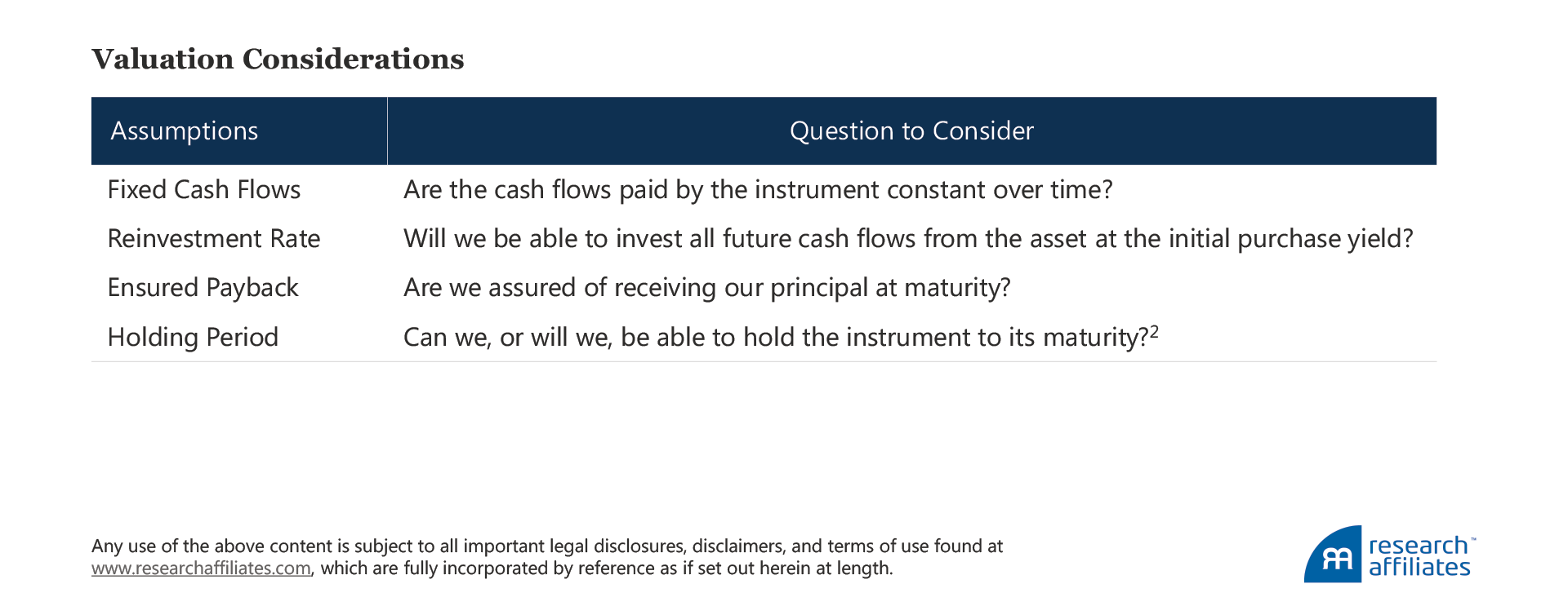
The challenge arises once we price a wider variety of instruments, which inevitably forces us to answer “no” to one or more of these questions. Doing so moves the expected return away from the purchase yield and requires a more-complex model. As a result, expected return is far more difficult to estimate, and the probability of unexpected shocks increases. To help tackle this reality, we use a framework based on long-term expectations.
Begin with a Focus on the Long Term
To reduce the impact of idiosyncratic shocks that occur in asset returns, we focus on long-term returns because, historically, the more returns that are averaged together, the tighter the distribution. My intent with this point is not to introduce a debate on mean reversion, but simply to acknowledge the data we have historically observed across markets. For example, over the last 140 years in the US equity market, Aked and Ko (2017) show that, for a 1-year horizon, the volatility of returns has been 19.2%, while at a 10-year horizon, the volatility dropped to 4.7%.3
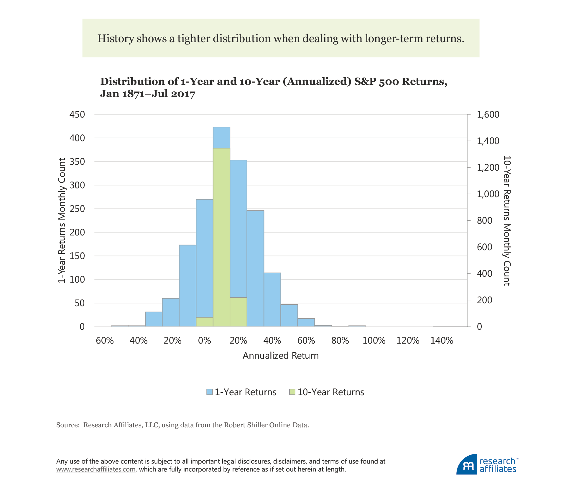
Armed with these historical data, we can feel confident that a 10-year expected return will have a fairly tight distribution when compared to its shorter-term counterpart of a 1-year expected return. But unless an investor is comfortable accepting the historical average return as the expectation for the future, something we’ve written extensively about as being a bad idea, a tighter distribution of historical10-year returns does nothing to help us understand the expected return (mean) of this distribution. For that, we must turn to another asset characteristic, return relationship.
Forecasting Bond Returns
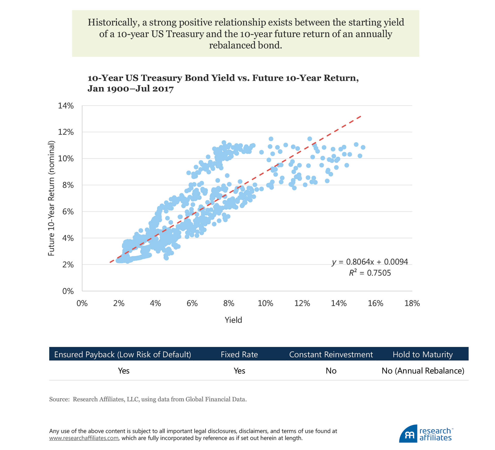
As noted earlier, the process of calculating an asset’s expected return is related to how much we must relax assumptions of quality, cash flows, reinvestment rate, and holding horizon. To better understand this framework, let’s look at an example of a 10-year fixed-rate US Treasury bond (historically, without default) and compare the purchase yield to the total nominal return.4
To make a more interesting example, let’s consider a 10-year fixed-rate coupon-paying US Treasury bond, but instead of holding the bond to maturity, we create a pseudo-constant 10-year maturity bond. For this investment, we purchase a 10-year US Treasury, hold it for one year, at which point we sell the now 9-year bond to purchase a new 10-year bond. Referring to our framework, we are relaxing the hold-to-maturity and constant reinvestment rate assumptions. Doing so, we still observe a strong positive relationship, an R2 of 75% and a coefficient close to 1.
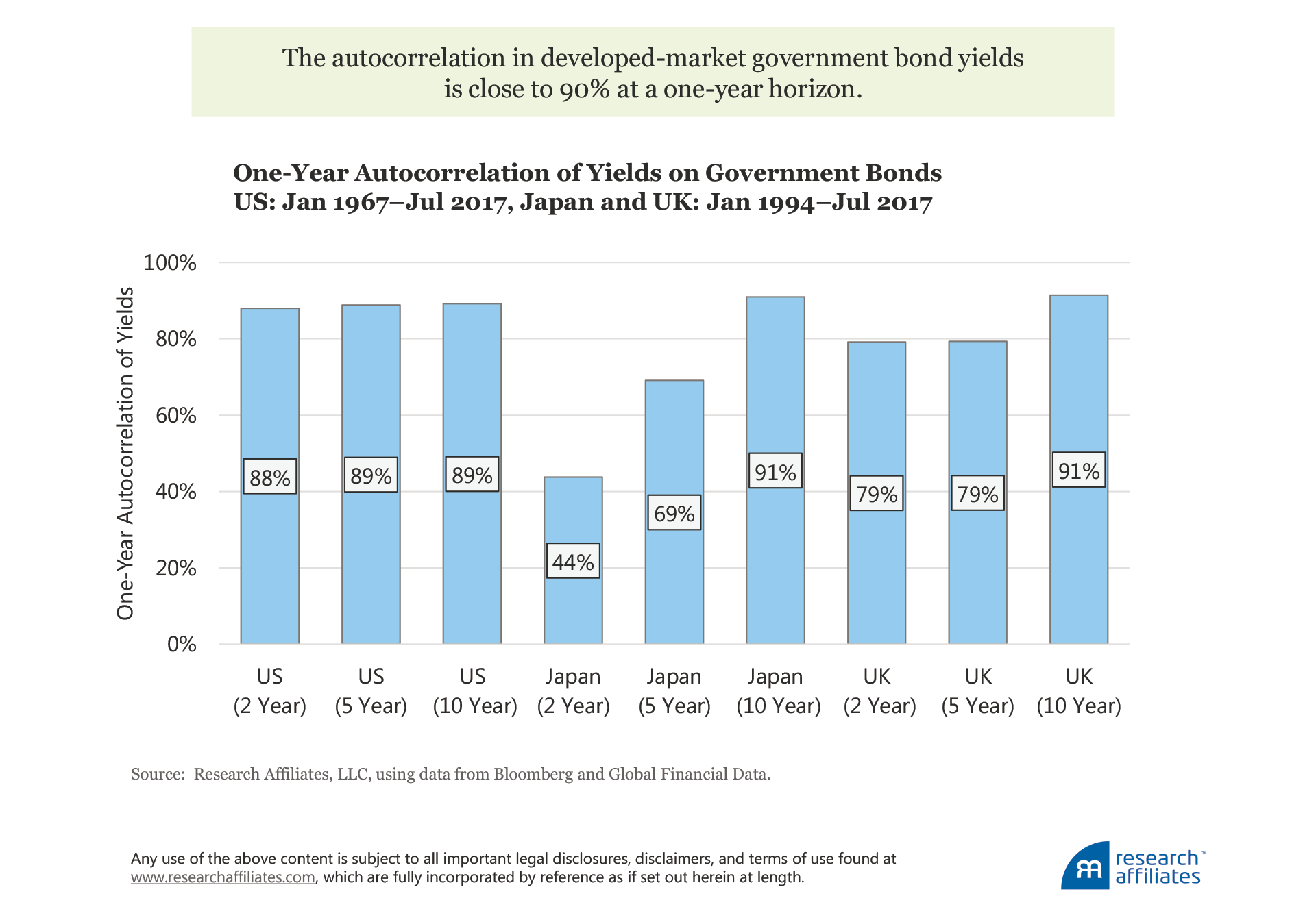
This relationship will hold for any similar security; it is not inherently unique to US Treasury bonds. In fact, the important metric is the autocorrelation in yields, which for a number of developed-market government bonds is close to 90% at a one-year horizon. This means a strong relationship exists between the yield of a bond today and the yield of a similar bond issued one year ago. Therefore, if it is not possible to hold the bond to maturity, a “similar” instrument will typically be obtained by selling the bond owned after one year and purchasing a new bond having the original maturity (creating a pseudo-constant maturity instrument); in the earlier example, this involved selling the original 10-year maturity after one year and purchasing a new 10-year maturity.
Forecasting Stock Returns
Stocks, by their very nature, require us to relax each of our four initial assumptions or conditions. Equity holders are often wiped out by default, intermediate cash payments and reinvestment conditions change over time, and stocks do not have a predefined maturity date at which the investor’s principal is returned. For these reasons, we expect, and see, a much noisier relationship between an investor’s purchase yield and future return. At a 10-year investment horizon, however, a meaningfully positive relationship still exists, albeit with a greater amount of dispersion around the trend. Historically speaking, starting dividend yield has done a nice job of predicting future returns!
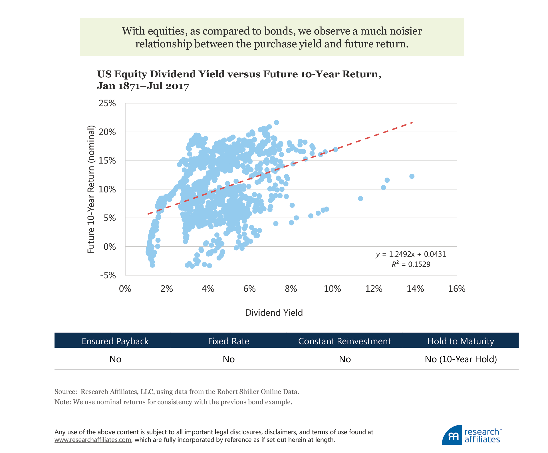
Does this mean we should rely on dividend yield alone to form our future expectation of return? Not really. Since 1871, the coefficient of dividend yield to return is, like bonds, close to 1, actually just a bit above. If we focus solely on the post-war period of January 1946 to July 2017, we see a similar relationship, but with a coefficient close to 3. Because investors don’t receive a quarterly check in the amount of $3 for every $1 of dividends paid by a company, the implication is that although simple yield is a good starting point, we should find a better way to estimate future return.
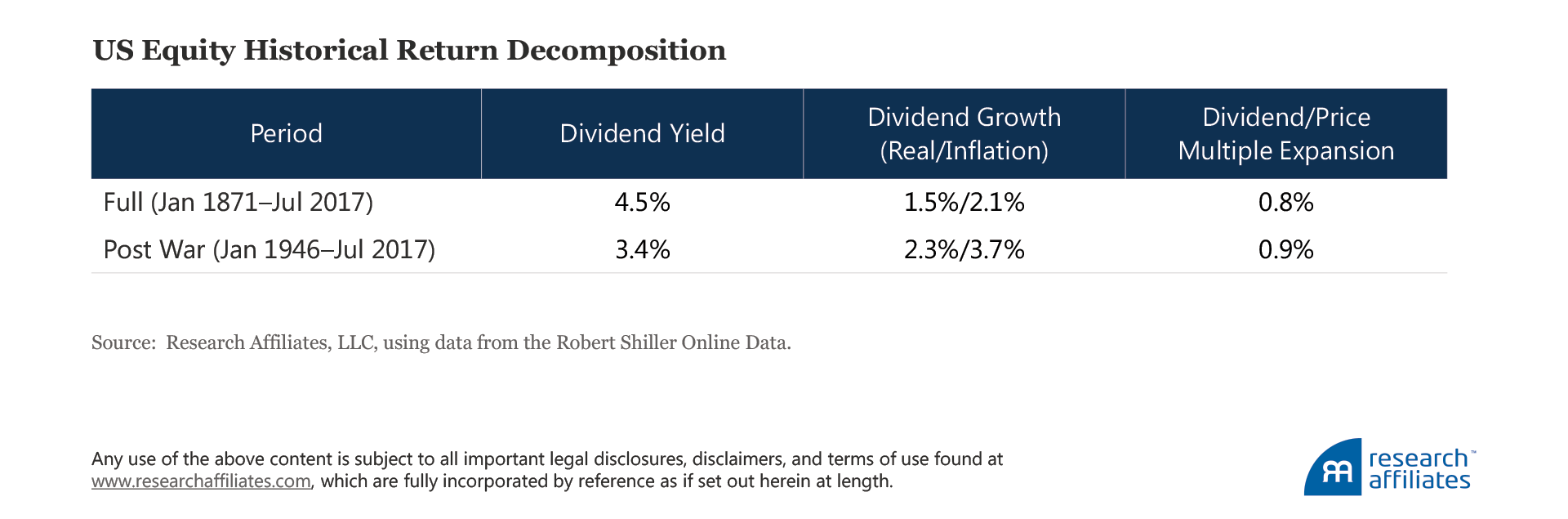
So, although dividend yields are a good starting point for deriving forward-looking estimates, we also need to consider other potentially meaningful sources of return. Through a simple decomposition of stock returns over the last two centuries, we can identify three reliable components to forecast and model (Arnott and Bernstein, 2002). In short, depending on the time span, nearly one-third to one-half of the long-term return on stocks comes from sources other than dividend yield, such as inflation, growth in dividends, and changes in valuation levels. We are able to extend this framework beyond US stocks to any asset class which relaxes the constraints in a similar way.
For those familiar with the Asset Allocation Interactive tool on our website, these three decomposition components will no doubt look familiar as the building blocks of return we incorporate in the tool. They come from a simple rearrangement of the terms in the equation used to calculate return (see Baetji and Menkhoff [2016] for a full derivation):

More Complete Model
Adding more terms to our expected return model requires us to generate a forecasting model for each. In addition to dividend yield at each point in time, we use the long-term growth in real earnings per share to forecast cash flow growth, and the reversion in the Shiller P/E multiple for expected changes in the cash flow multiple. For expected returns, because the return from inflation is lost due to reduced purchasing power, we prefer to focus on expectations of return, net of inflation.
The Gordon Growth Model focuses on a constant-future-yield framework and only includes yield and growth as drivers of future return. Whereas the industry continues to debate the efficacy of Shiller P/E reversion, we at Research Affiliates firmly believe in mean reversion in asset prices (Brightman, Masturzo, and Treussard, 2014), although we acknowledge it to be tricky to accurately forecast. As the great Peter Bernstein (1996) once said about mean reversion:
First, it sometimes proceeds at so slow a pace that a shock will disrupt the process. Second, the regression may be so strong that matters do not come to rest once they reach the mean…. Finally, the mean itself may be unstable, so that yesterday’s normality may be supplanted today by a new normality we know nothing about. (p. 172)
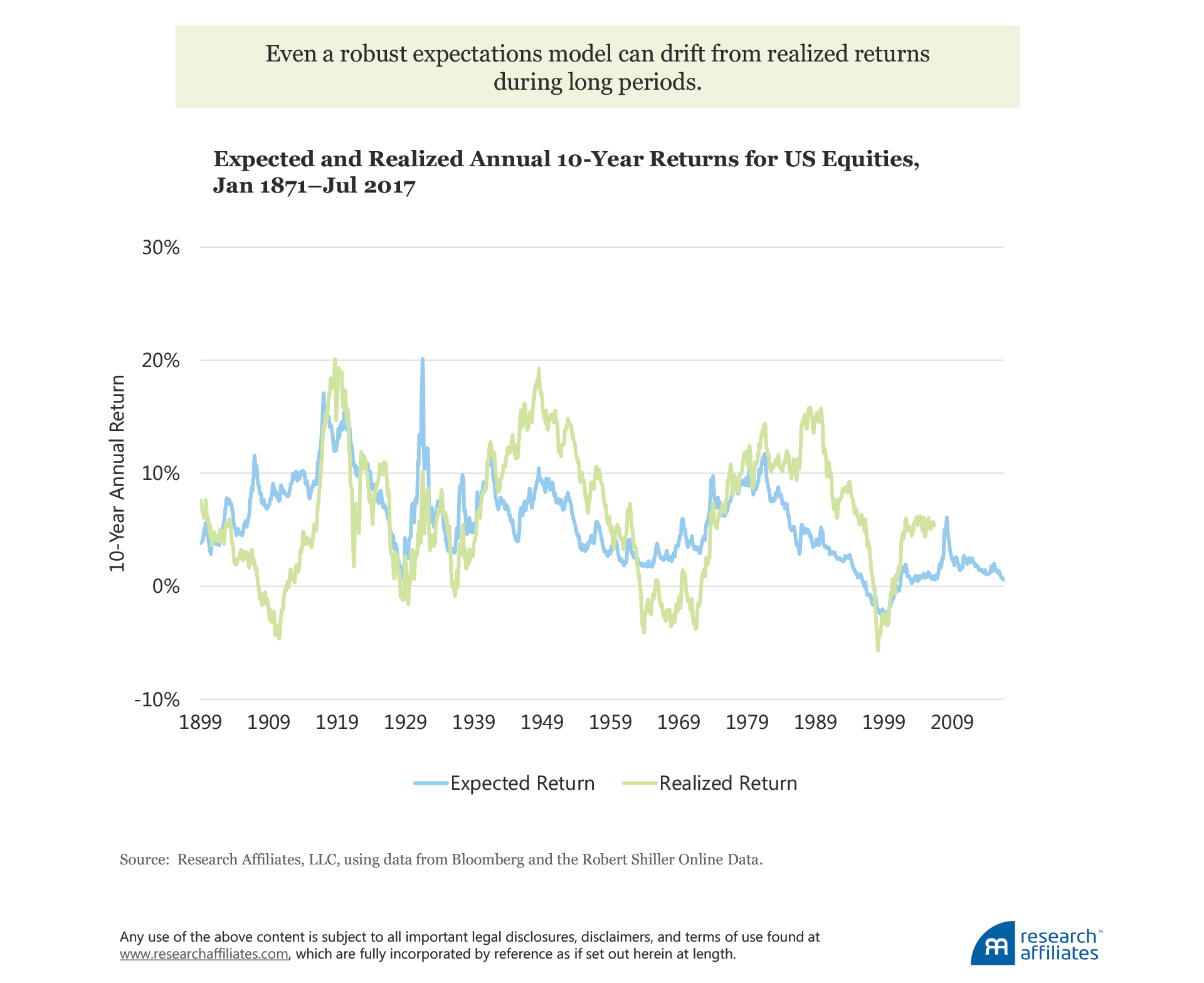
For the most part, the trend in our expectations of US stock returns has been in line with subsequent realized returns; however, sometimes (especially recently) we’ve missed the mark, sometimes by a lot, even with the benefit of hindsight. Drafting expectations of return is definitely not an exact science.
Even if our models sometimes misestimate realized return does not mean we should abandon the work of modeling expectations. Certainly, the attempt to construct an accurate future expected return is one goal in the modeling process, but another immensely important goal is using the model to create portfolios with value-add. Considering only the models for stocks and bonds so far introduced in this article, we can look at their value in the context of portfolio construction.
Building a Portfolio Using Expected Returns
Because the objective of investors is inevitably to create portfolios, expectations of risk and return can be viewed as signals to be used in achieving that end. Perhaps surprisingly, we don’t even need accurate expected returns versus future realized returns in order to generate value-add portfolios, those capable of outperforming a particular benchmark. We can demonstrate this in the context of a two-asset portfolio of US stocks and bonds. Restricting our case study to two assets is done for simplicity and to illustrate a point, not to imply that investors should ever restrict themselves simply to two assets.
A very common way to generate portfolio weights from risk and return expectations is through the use of mean-variance optimization (MVO), which aims to create the portfolios with the highest achievable return per unit of risk, also known as efficient frontier portfolios. Although the benefits of MVO are vast, the approach has a few important drawbacks, such as high sensitivity to our input expectations as well as difficulty in tying the resulting portfolio weights to the input expectations, especially when the number of assets grows. Thus, for our case study, let’s take a different, but very straightforward, approach.
Instead of comparing our risk and return expectations cross-sectionally among assets, à la MVO, let’s compare the current expected return for each asset against its own historical time series of expectations. In this way, we are attempting to neutralize some of the deficiencies (noise) in our models that we expect will be relatively constant over time. Through this comparison, we can derive a confidence score for each asset based on its expected return. For example, if an asset has a high expected return versus its expected return history, our model should show more confidence in the cheapness of that asset versus how the model has historically viewed it. It’s easy to understand why we would want to overweight that asset from its neutral position, or vice versa if the expected return is low. This approach is not new, and Asness, Ilmanen, and Maloney (2015) discuss a very similar approach.
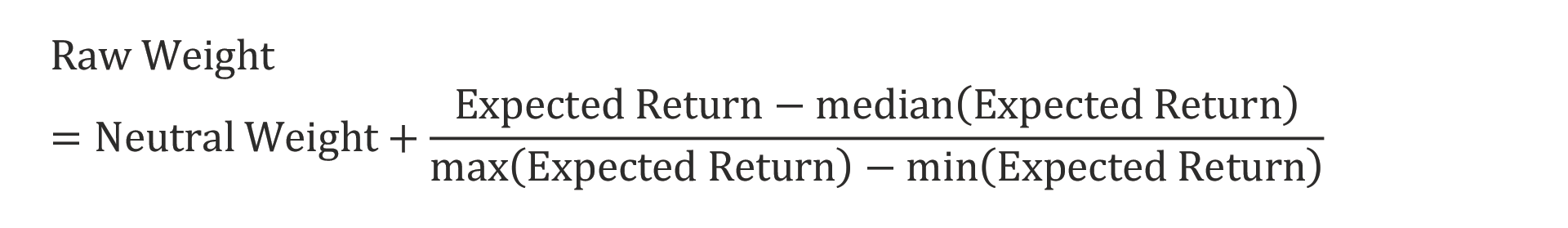
The first step is to create a confidence score (i.e., raw weight) for each asset5 by comparing the current expected return to its historical median using a variant of standard min–max scaling. The confidence score then indicates the amount of the over- or underweight compared to the neutral position. The following equation shows that if the current expected return is higher than the historical median, the raw weight implies an overweight to the asset, or if less, an underweight:
Because we are comparing our simple strategy to the traditional 60/40 portfolio, we set the neutral weights in our portfolio to 60% for stocks and to 40% for bonds. Having tested other neutral weights against their respective benchmarks, we find they produce similar results.
Thus far, we have considered each asset in isolation, ignoring all cross-sectional relationships, which is not to imply they are not important, they definitely are. In this framework, cross-sectional relationships are introduced through weight normalization; the portfolio must be fully invested in the two assets and not take on leverage. We may want to overweight both assets, overweight one and underweight the other, or underweight both based on the assets’ current expected returns versus their respective histories. By normalizing the weights for full investment, those with higher scores will get higher allocations, and vice versa, thus introducing a cross-asset comparison of expectations.
In our example, data begin in 1910 in order to have 20 years to develop an earnings growth rate for stocks’ expected returns and another 10 years to capture the statistics necessary to calculate the raw weight. By doing so, our expected returns only contain information available at each point in history.6
Because we are interested in 10-year expected returns, it makes sense to set our rebalance period for the portfolio at 10 years. Otherwise, we would be giving up information contained in our expected return models. For shorter rebalance periods, we would use shorter-horizon expectations, although in this case, we only have long-horizon returns. Therefore, let’s “cheat just a little” and use a 5-year rebalance period, which balances the usefulness of the portfolio with consistency in the horizon of the expectations.
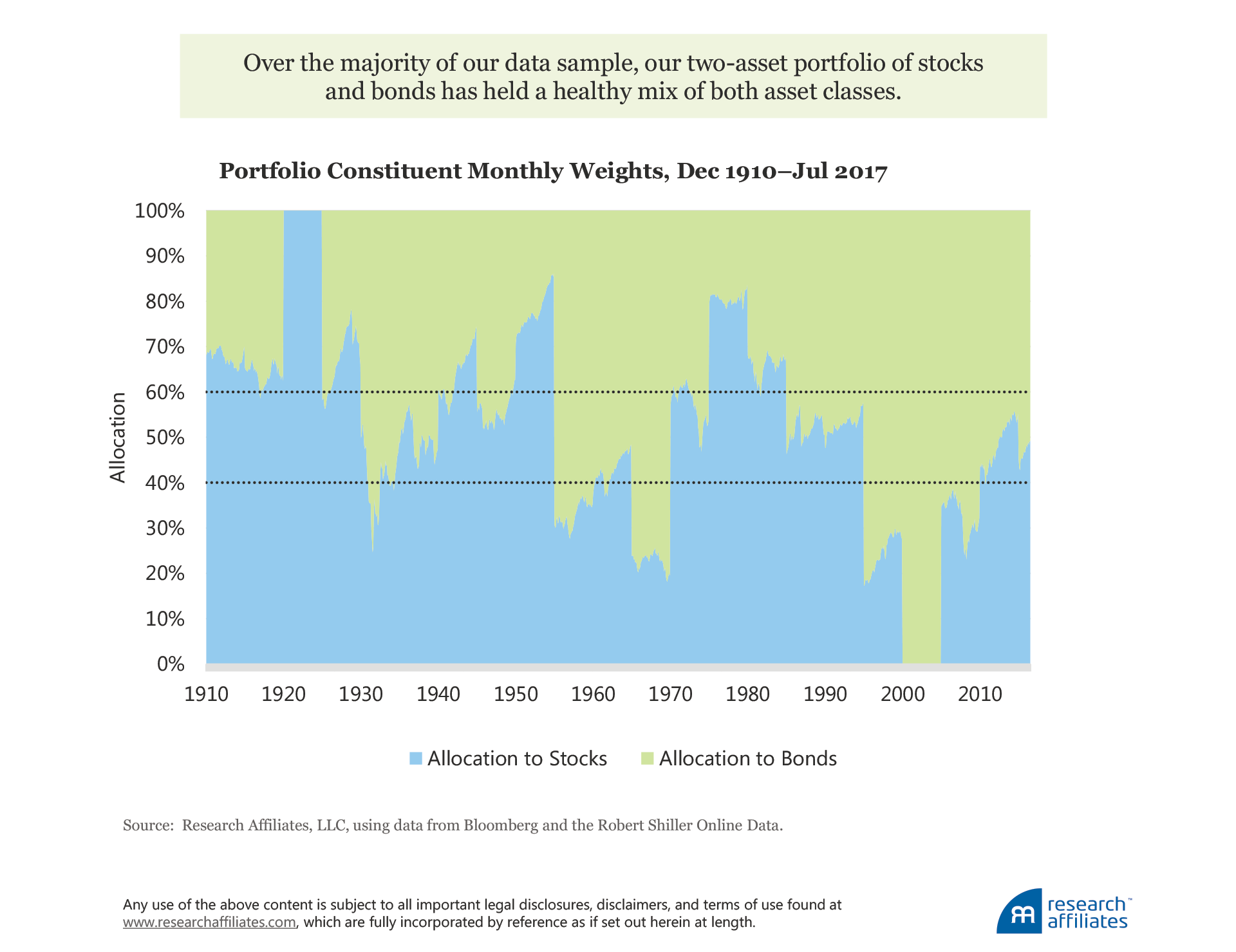
Over our data sample, two periods existed in which the portfolio was 100% invested in a single asset. In the early 1920s, the portfolio was 100% invested in stocks, whereas in the early part of the current century, it was 100% invested in bonds. The majority of the time, however, our portfolio has held a healthy mix of both assets. For example, starting in the 1960s and through the inflationary 1970s, the portfolio loaded up on stocks and sold bonds, before reversing course through the 1980s and 1990s. More recently, the strategy views both stocks and bonds as expensive and has been moving toward a more neutral 60/40 weight.
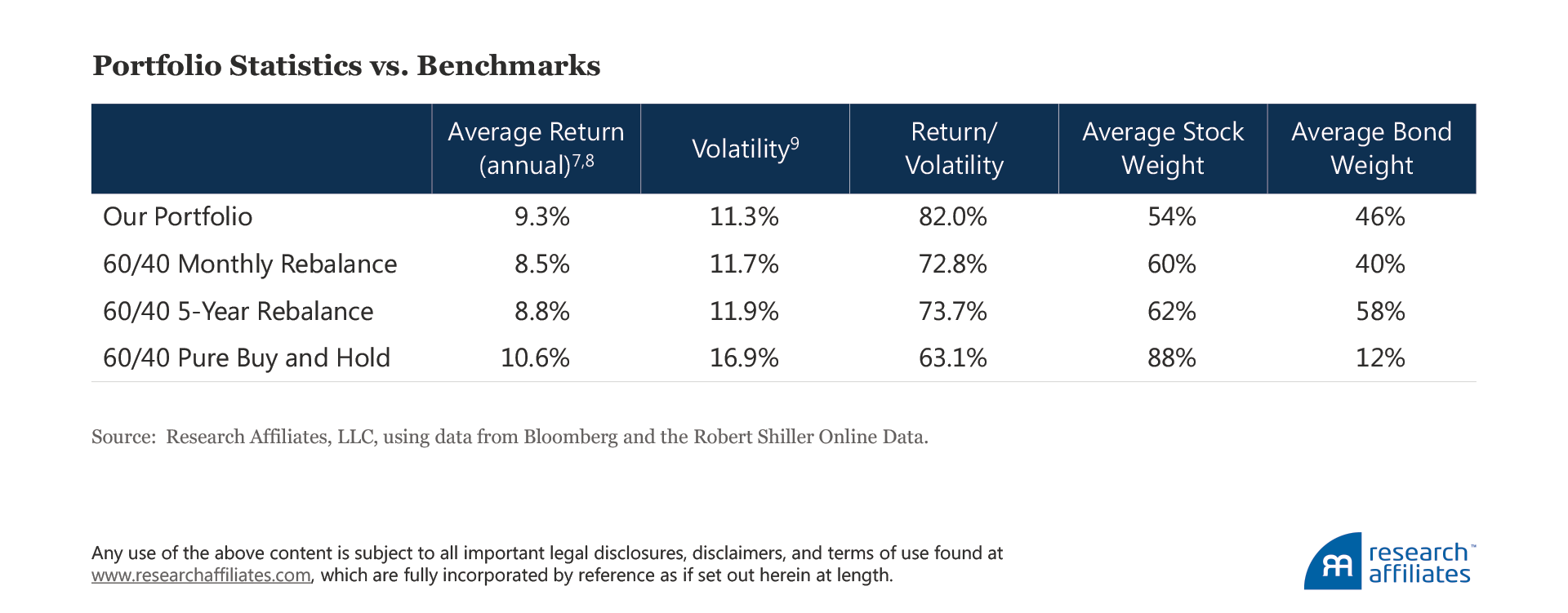
This simple trading strategy outperforms a 60/40 portfolio, regardless if the latter is rebalanced on a monthly basis, a five-year basis, or not at all (a pure buy-and-hold strategy). In addition, risk-adjusted outcomes improve, even while, on average, maintaining a lower exposure to US equities, the dominant risk exposure in most investors’ portfolios.
What This Means
Our multi-question valuation framework provides a tested approach for generating future values of any asset class. Importantly, it also propels us to examine underlying core assumptions and question how asset classes inherently relax some or all of the four conditions. In this article, as we have studied and applied this framework using the two most common asset classes—stocks and bonds—to build a simple portfolio. In doing so, we are reminded of a few enduring principles.
First, our framework does not by any means imply that the expected outcomes will be close to—let alone, consistently match—future realized returns, especially over short time horizons. In our industry, a focus on achieving short-term accuracy is tempting. But deriving forecasts can give a false illusion of precision and statistical clarity. Like most managers, we have no special skill or clairvoyance in predicting the short term. As such, we take advantage of historic long-term relationships to generate our long-term expected returns.
Second, although the example in the article has focused exclusively on stocks and bonds, the concepts underlying our framework apply to any asset class. The beauty of the simplest of frameworks, such as the one we use here, is that it clearly forces us to understand how each asset relates to key assumptions. For asset classes that relax all criteria, we can then understand how to improve and expand our framework to better inform long-term expected outcomes.
Finally, even if our long-term expected returns meaningfully diverge at various times from realized returns—a fact that every investor must not only be aware of, but expect—it doesn’t mean our process is broken or unproductive. Creating a rich set of expected return models enables us to create portfolios capable of outperforming, even if the asset models themselves are operating with low accuracy over certain periods.

Endnotes
1. From a letter sent in 1703 by Gottfried Leibniz (1646–1716), a German mathematician and philosopher, to Jacob Bernoulli (1654–1705), a Swiss mathematician who made significant contributions in the field of probability.
2. Many reasons exist for an investment not to be held to maturity, some due to the investor and some to the issuer. A few of these reasons include the instrument’s maturity is longer or shorter than the investment horizon, the instrument is paid back early, or the issuer recalls the instrument.
3. Aked and Ko (2017) also point out that investors should be aware that although the average volatility over a decade is low, which is meaningful for generating expectations of return, over a 10-year period investors will experience, on average, 14.9% volatility each year.
4. We use nominal returns because the bond yield is stated in nominal terms and includes an expected market inflation rate. The relationship of yield to the real return of bonds is much weaker because the market-implied inflation rate at the purchase date could be vastly different from realized inflation over the 10-year horizon. Also, as noted earlier, if the bond was a zero-coupon bond, held for 10 years, the return would be the same as the starting yield, a perfect correlation.
5. For implementation, we replace the minimum expected return with the 5th percentile rank and the maximum expected return with the 95th percentile rank, consistent with Asness, Ilmanen, and Maloney (2015).
6. Although we readily concede that no backtest can ever truly be out of sample when using data from the past known to the modeler at the time the model is created.
References
Aked, Michael, and Amie Ko. 2017. “Time Diversification Redux.” Research Affiliates (August).
Arnott, Robert, and Peter Bernstein. 2002. “What Risk Premium Is ‘Normal’?" Financial Analysts Journal, vol. 58, no. 2 (March/April):64–85.
Asness, Cliff, Antti Ilmanen, and Thomas Maloney. 2015. “Market Timing Is Back in the Hunt for Investors.” Institutional Investor (November 11).
Baetje, Fabian, and Lukas Menkhoff. 2016. “Equity Premium Prediction: Are Economic and Technical Indicators Unstable?” DIW Berlin Discussion Paper No. 1552 (February 24). Available at SSRN.
Bernstein, Peter. 1996. Against the Gods: The Remarkable Story of Risk. New York, NY: John Wiley & Sons, Inc.
Brightman, Chris, Jim Masturzo, and Jonathan Treussard. 2014. “Our Investment Beliefs.” Research Affiliates (October).
